Syllabus
Eight modules, from roots to differential equations
The course follows a first university course in numerical analysis. All eight modules are complete.
-
01Lectures 1–7 Available
Root finding
Bisection, secant, regula falsi, Newton, fixed-point iteration, order of convergence
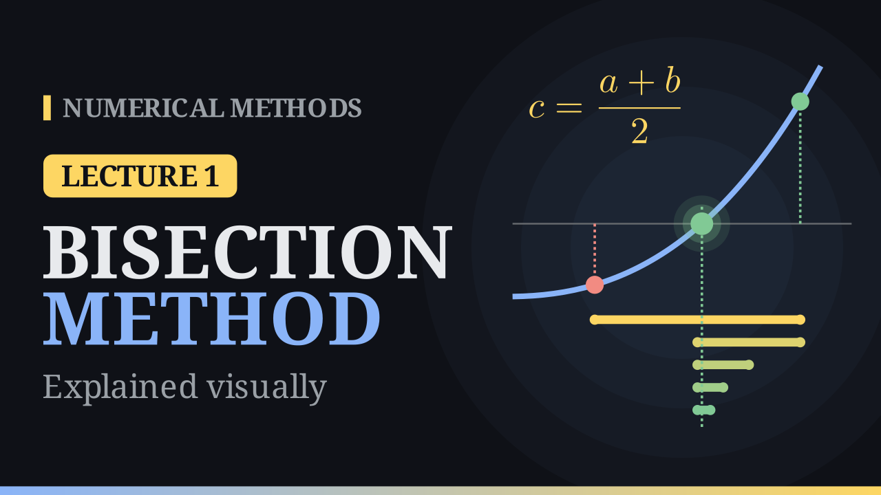 6:38
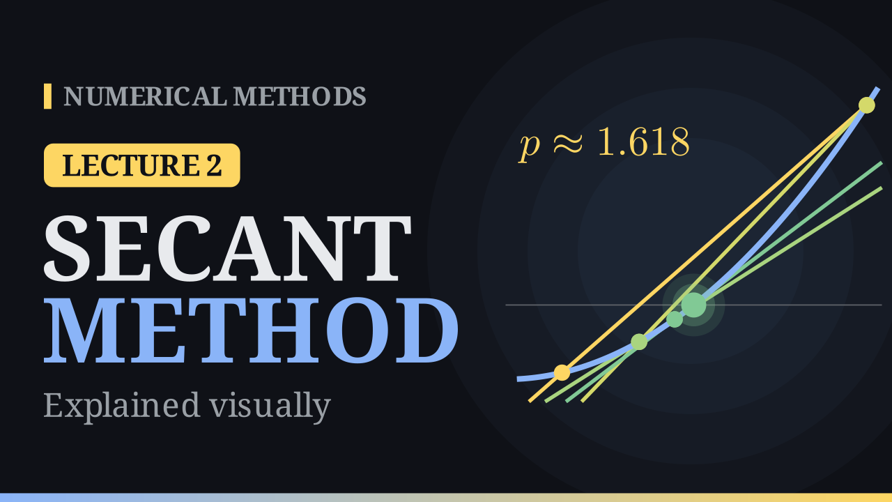 7:46
Lecture 2
The Secant Method
Replace the curve by a line through two points. Order 1.618, the golden ratio.
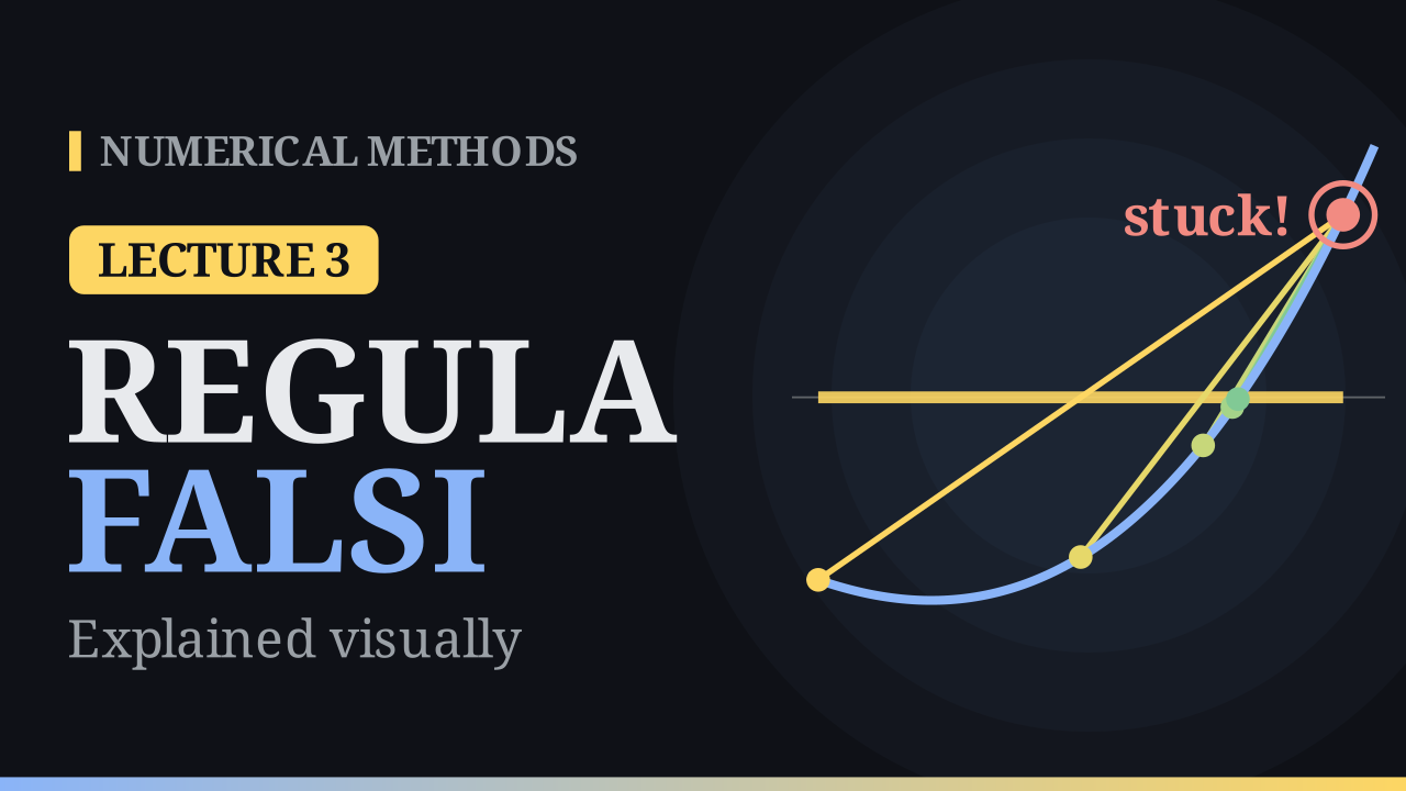 7:07
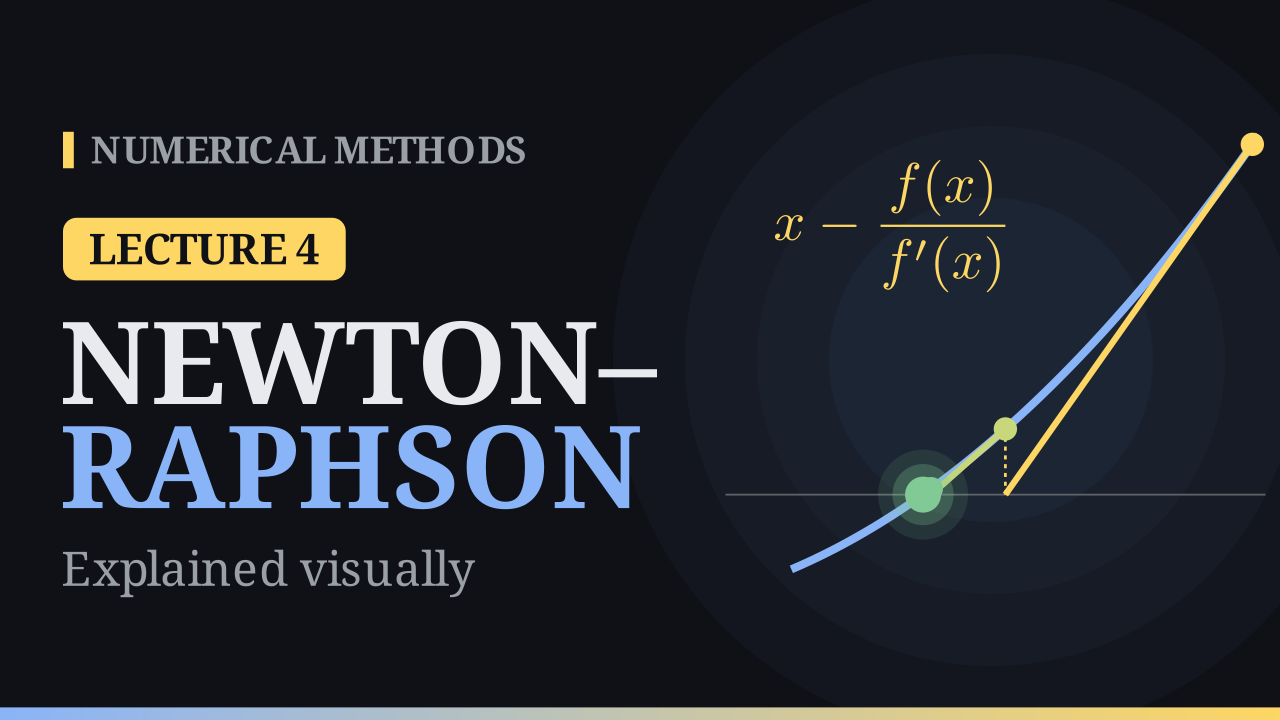 7:31
Lecture 4
The Newton–Raphson Method
Follow the tangent to the axis. Quadratic convergence and its failures.
 7:07
Lecture 5
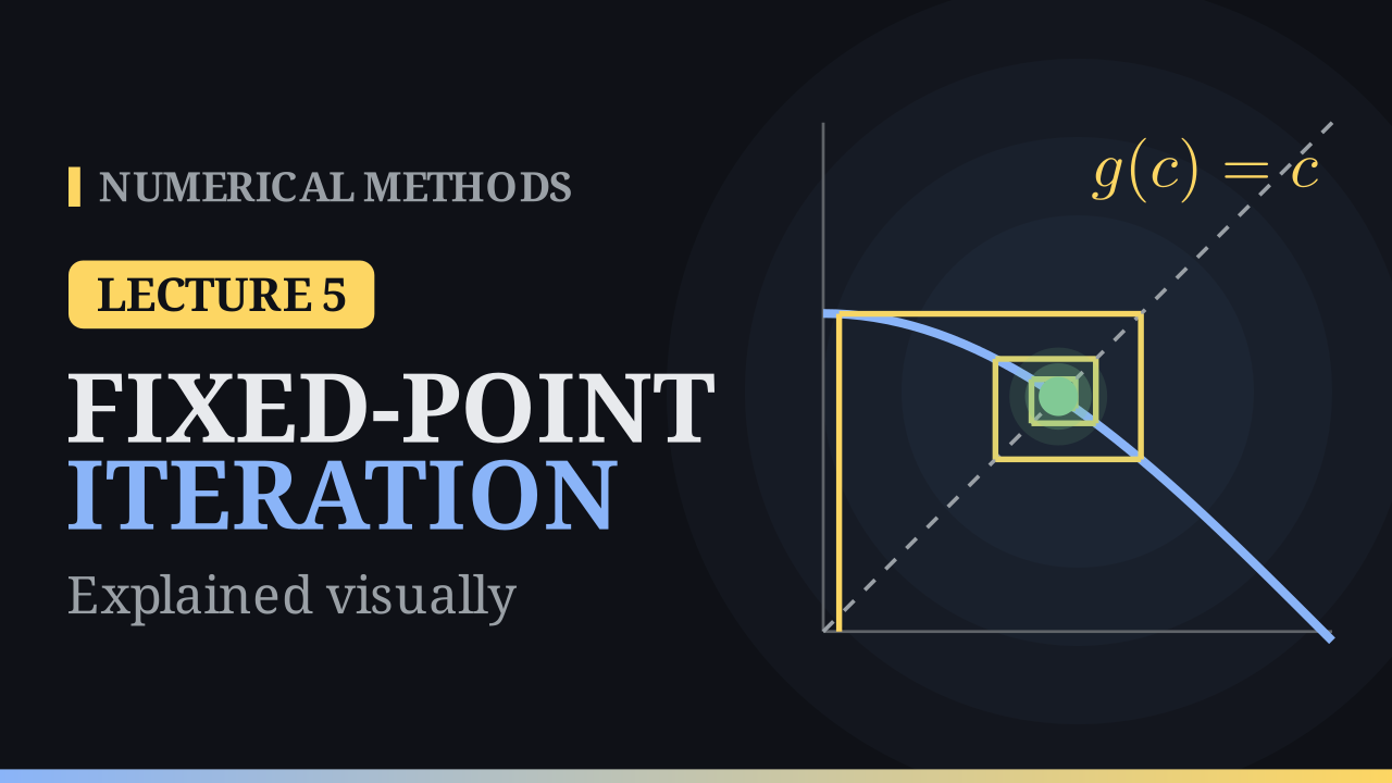
Fixed-Point Iteration
Rewrite f(x) = 0 as x = g(x) and read the behaviour off a cobweb diagram.
 7:25
Lecture 6
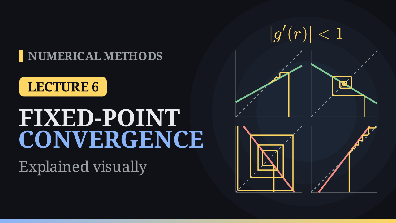
Convergence of Fixed-Point Iteration
Contraction mappings, error bounds, and the rate |g′(r)|.
 7:47
Lecture 7
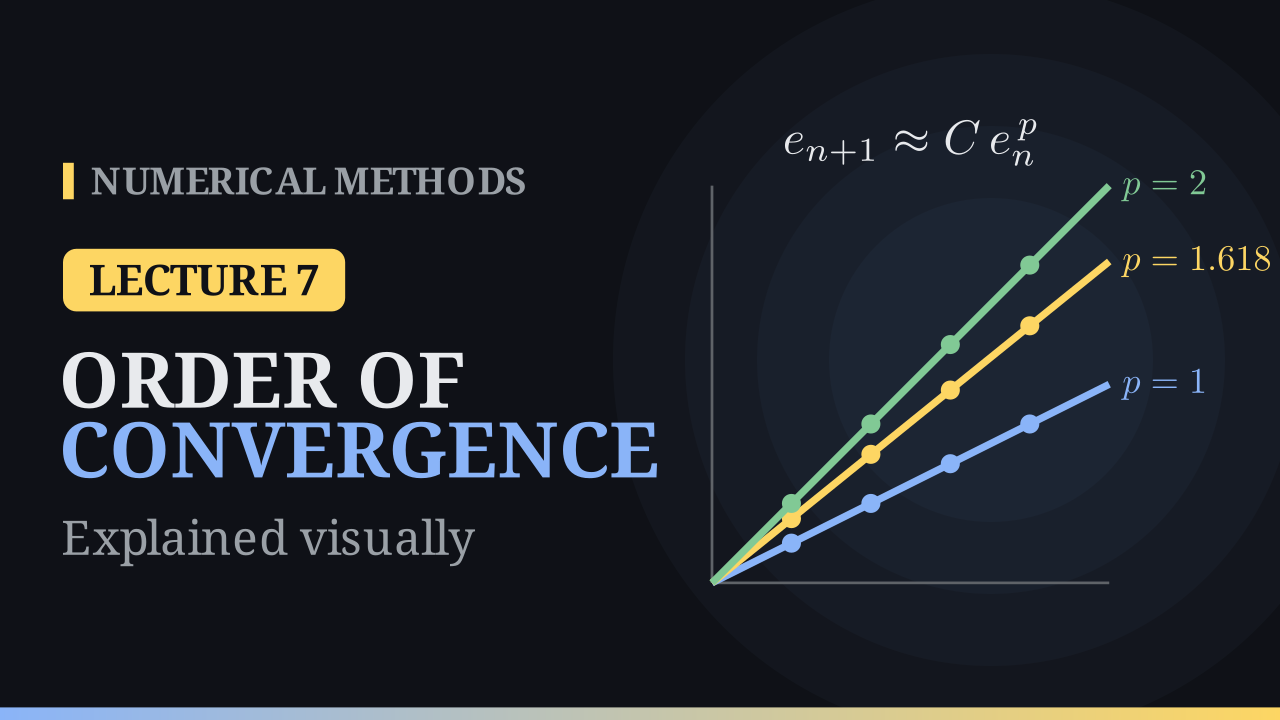
Order of Convergence and Modified Newton
Measuring the order p, multiple roots, and restoring quadratic speed.
-
02Lectures 8–9 Available
Computer arithmetic
Errors, floating-point numbers, machine epsilon, loss of significance
 8:44
Lecture 8
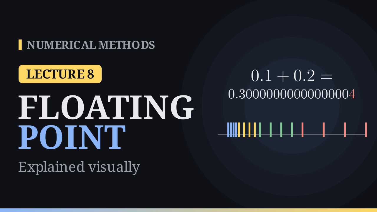
Errors and Floating-Point Numbers
Why 0.1 + 0.2 is not 0.3: binary, floating-point systems, chopping and rounding.
 8:56
Lecture 9
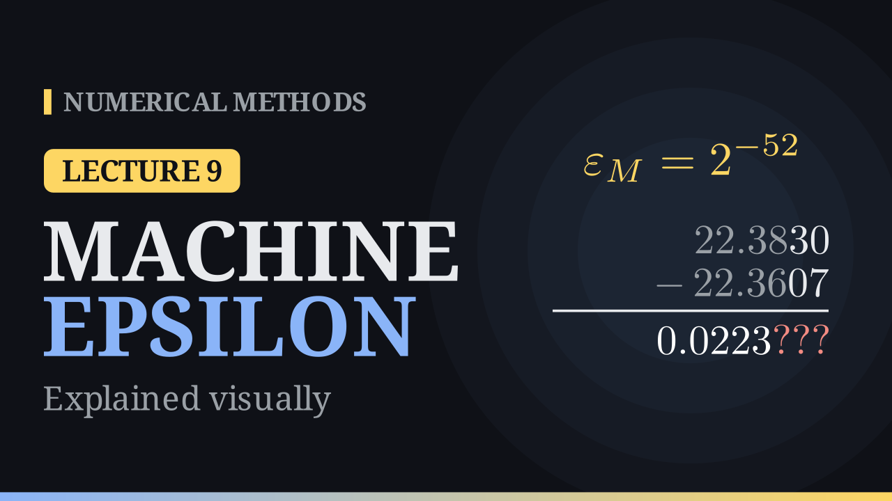
Machine Epsilon and Loss of Significance
Machine epsilon, catastrophic cancellation and how to avoid it, IEEE 754.
-
03Lectures 10–20 Available
Linear systems
Gaussian elimination, pivoting, LU and Cholesky, norms, conditioning, iterative methods
 7:20
Lecture 10
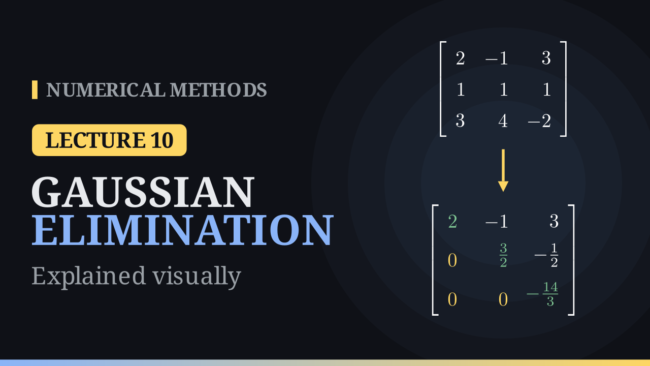
Gaussian Elimination
Row operations, back substitution, pivots and the determinant, and when elimination fails.
 7:33
Lecture 11
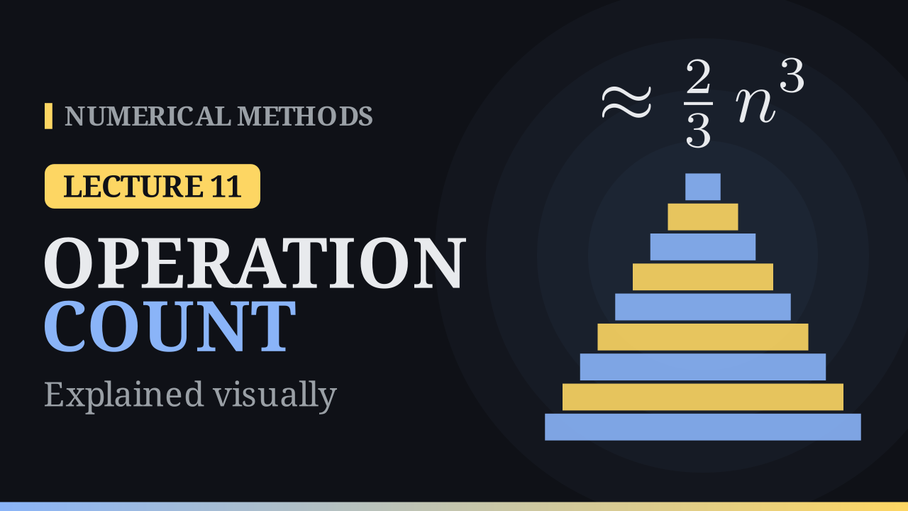
Operation Count of Gaussian Elimination
Why elimination costs about two-thirds n cubed, and why Cramer's rule and inverses are wasteful.
 7:49
Lecture 12
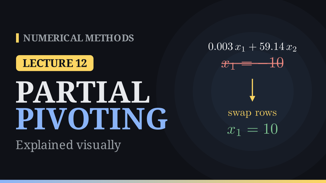
Partial and Complete Pivoting
Why small pivots ruin elimination, and how row and column swaps make it safe.
 9:21
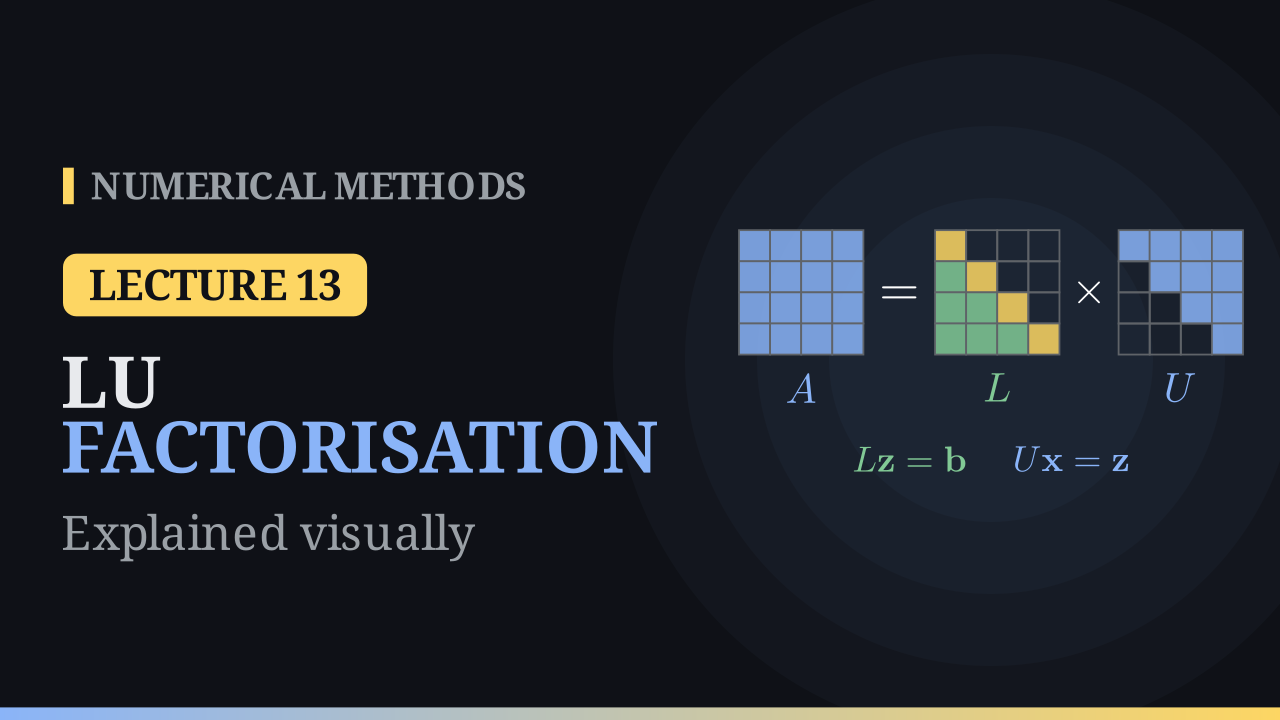
Lecture 13
LU Factorisation
Keep the multipliers of elimination: A = LU, two triangular solves, Doolittle, Crout and PA = LU.
 7:31
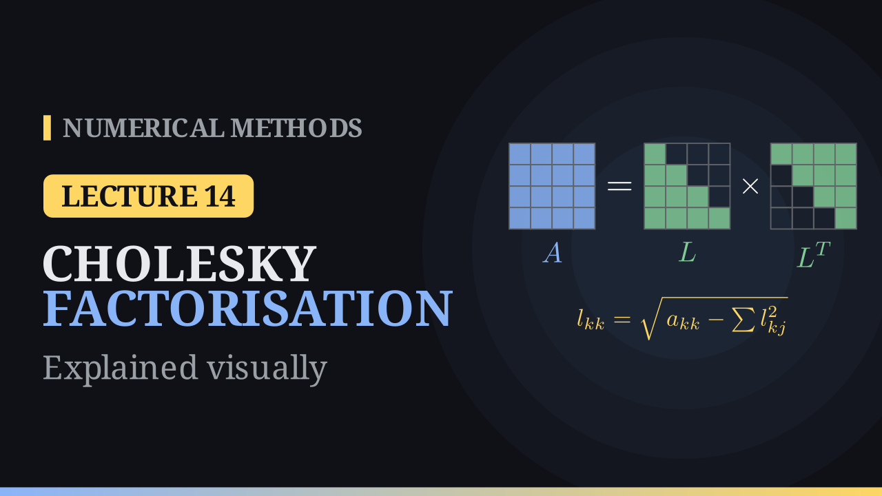
Lecture 14
Cholesky Factorisation
Symmetric positive definite matrices: A = LLᵀ at half the cost of LU, with no pivoting.
 7:53
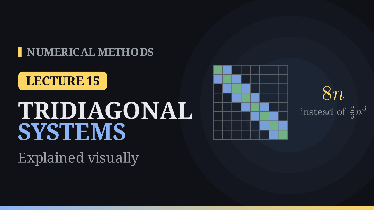
Lecture 15
Systems with Simple Structure
Diagonal, triangular and tridiagonal systems: back substitution and the Thomas algorithm in 8n operations.
 7:39
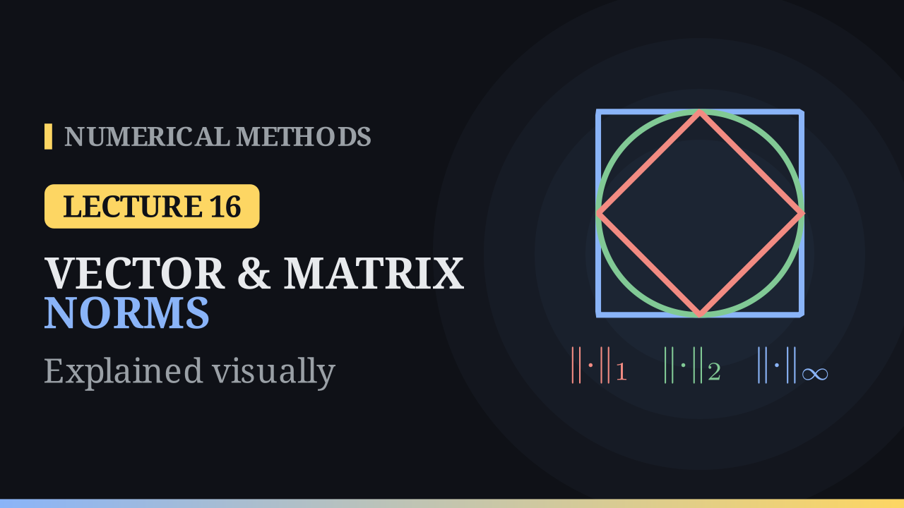
Lecture 16
Vector and Matrix Norms
Measuring vectors and matrices: taxicab, Euclidean and max norms, unit balls, and induced norms as the biggest stretch.
 7:37
Lecture 17
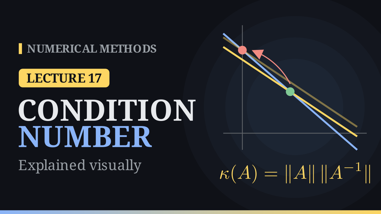
Sensitivity and Condition Number
Why tiny changes in b can ruin x: the condition number, lost digits, Hilbert matrices and the residual trap.
 7:25
Lecture 18
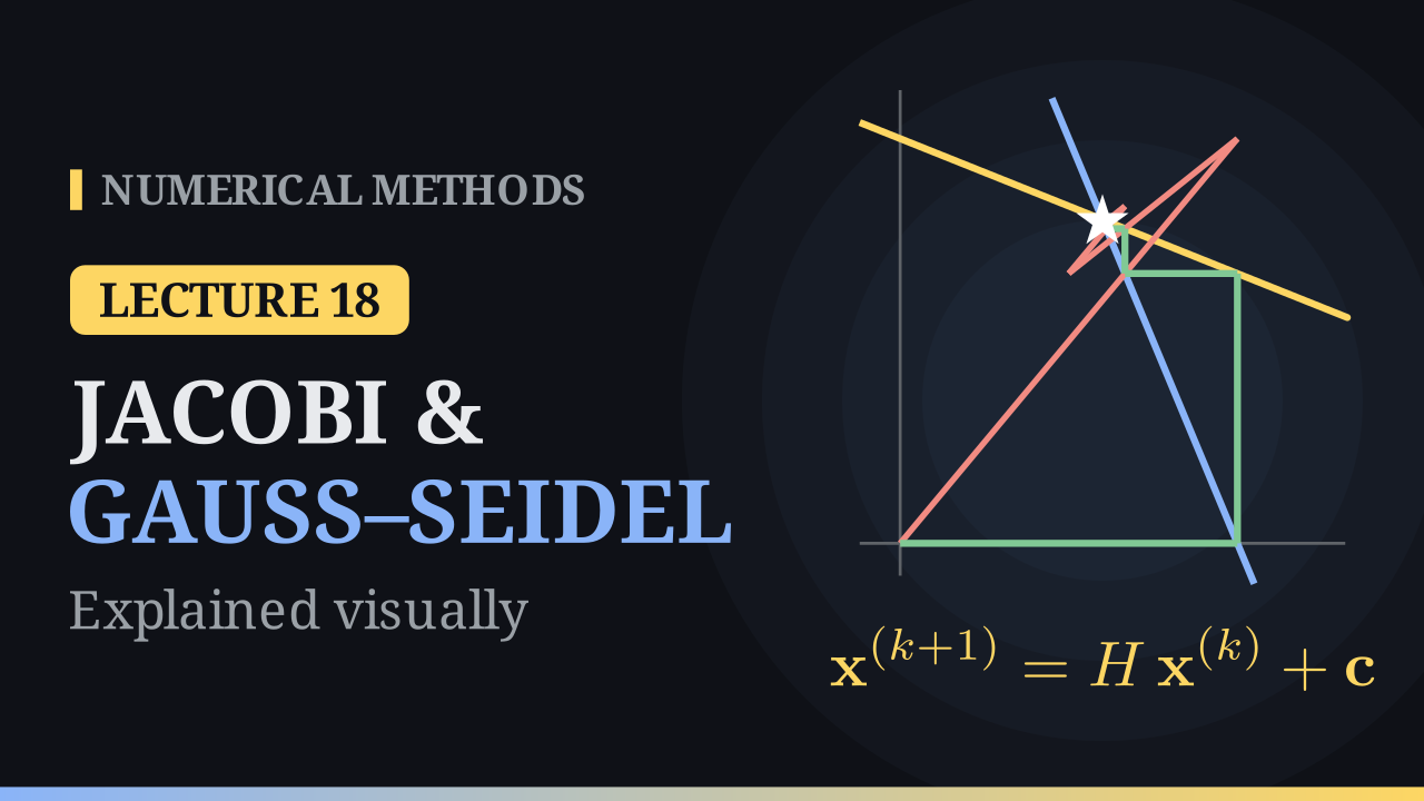
Jacobi and Gauss–Seidel Methods
Solving big systems by iteration: Jacobi's zig-zag, the Gauss–Seidel staircase, and diagonal dominance.
 7:34
Lecture 19
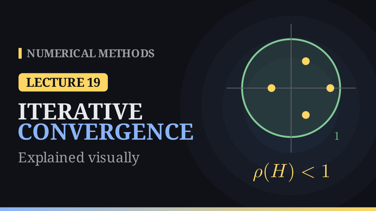
Convergence of Iterative Methods
Splittings, the iteration matrix and the spectral radius: when iterations converge and how fast.
 7:14
Lecture 20
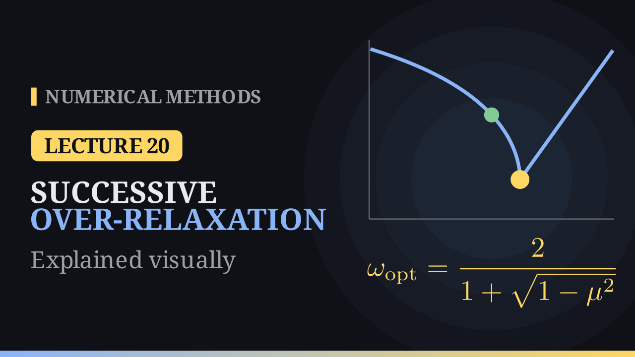
Successive Over-Relaxation (SOR)
One extra parameter ω: Kahan's bound, Young's optimal ω, and 7278 sweeps cut to 113.
-
04Lectures 21–23 Available
Eigenvalues
The power method, inverse and shifted inverse power methods
 8:05
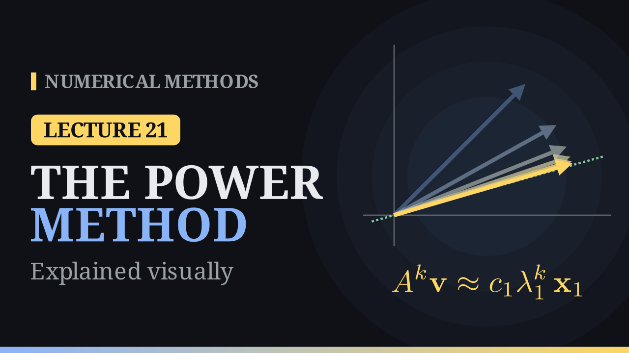
Lecture 21
The Power Method
Multiply by A again and again: the vector swings to the dominant eigenvector, at rate |λ₂/λ₁|.
 7:39
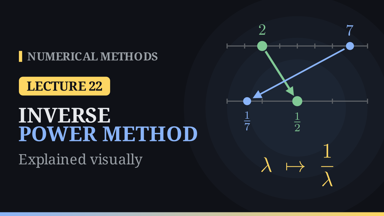
Lecture 22
The Inverse Power Method
Run the power method on A⁻¹ with one LU factorisation to find the smallest eigenvalue.
 7:53
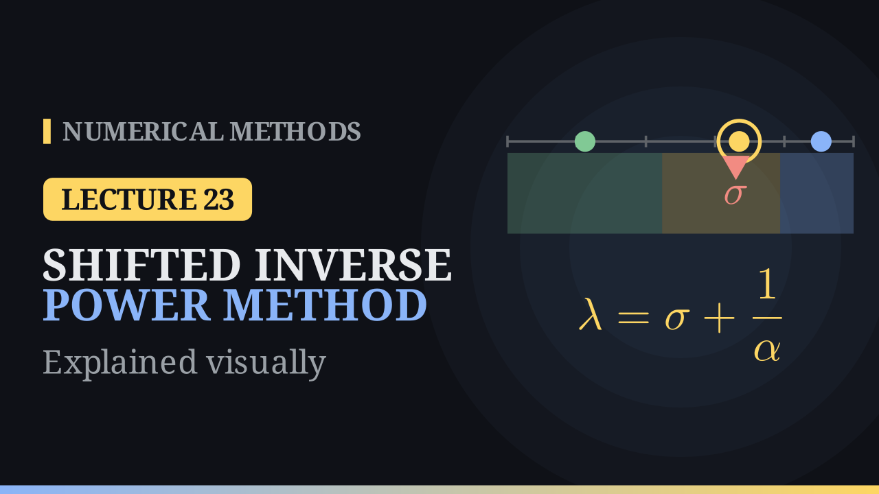
Lecture 23
The Shifted Inverse Power Method
Shift the spectrum to reach any eigenvalue, fast, and meet Rayleigh quotient iteration.
-
05Lectures 24–25 Available
Least squares
Fitting lines and polynomials to data
 7:34
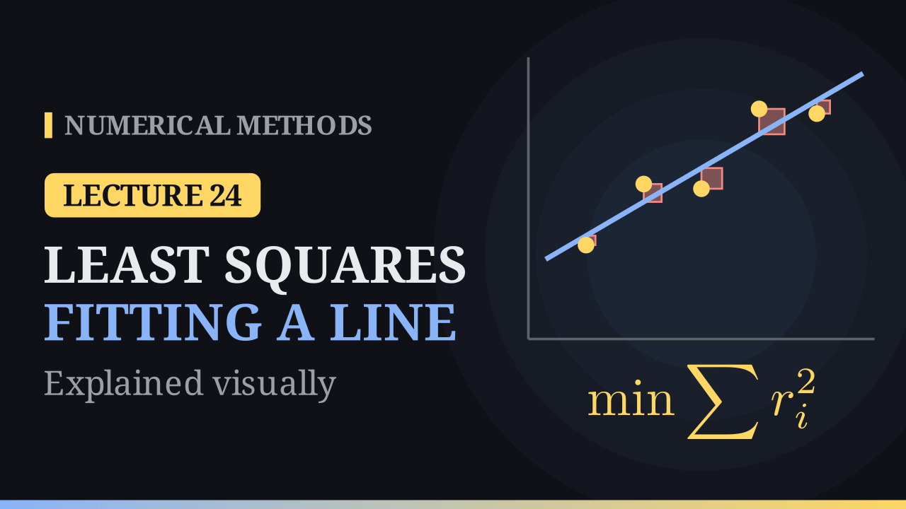
Lecture 24
Least Squares: Fitting a Line
Minimise the sum of squared residuals: the normal equations, the mean point, outliers and residual patterns.
 8:09
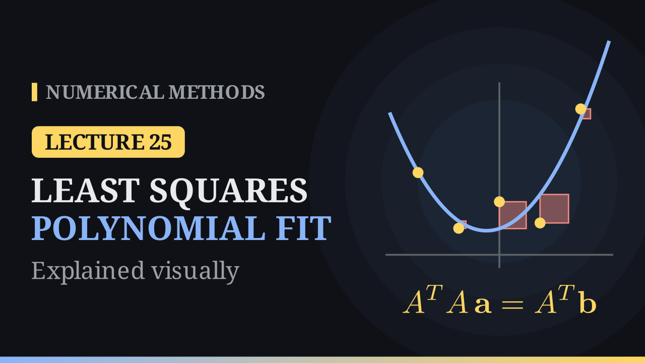
Lecture 25
Least Squares: Polynomial Fit
Fit polynomials of any degree with the normal equations, choose the degree, and linearise power laws.
-
06Lectures 26–29 Available
Interpolation
Lagrange and Newton forms, the error term, the Runge phenomenon
 9:48
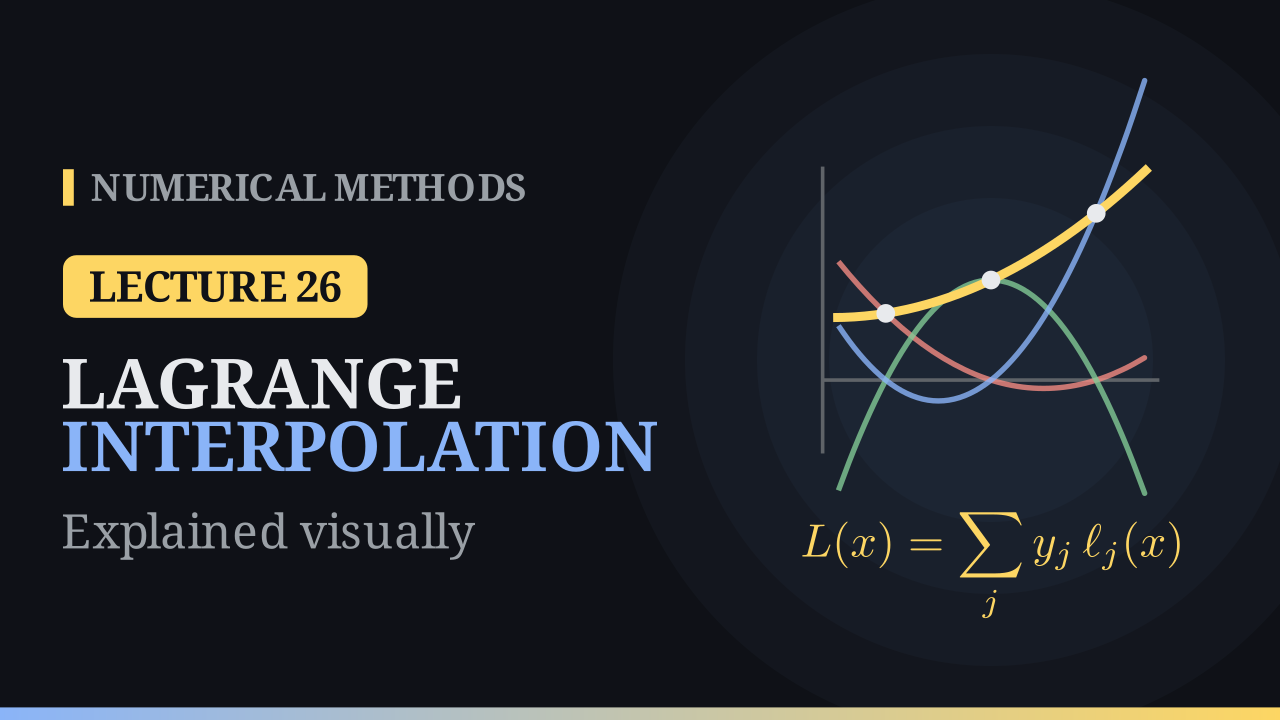
Lecture 26
Lagrange Interpolation
The one polynomial through every point: basis polynomials, scaled by the data and summed into the interpolant.
 10:05
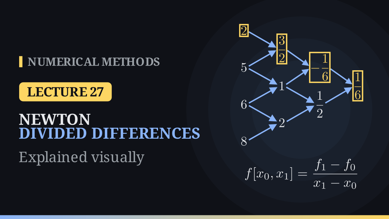
Lecture 27
Newton Divided Differences
Build the interpolant one term at a time from a divided difference table, add a point cheaply, evaluate by nesting.
 9:27
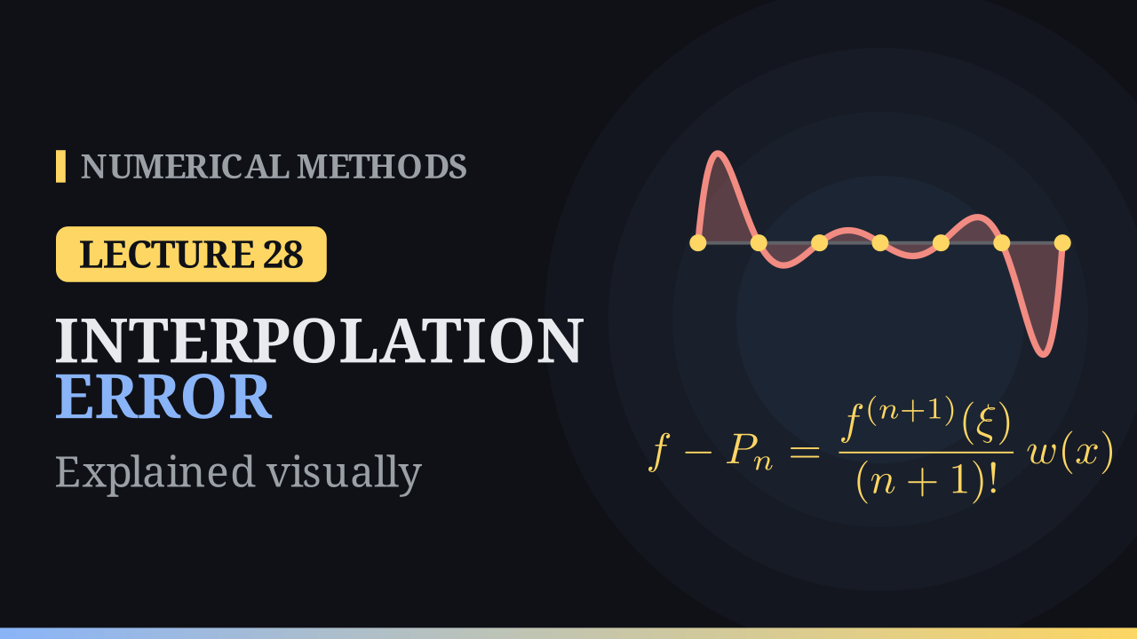
Lecture 28
The Interpolation Error
The error formula via Rolle's theorem, the node polynomial, and computable bounds such as h squared over 8.
 9:59
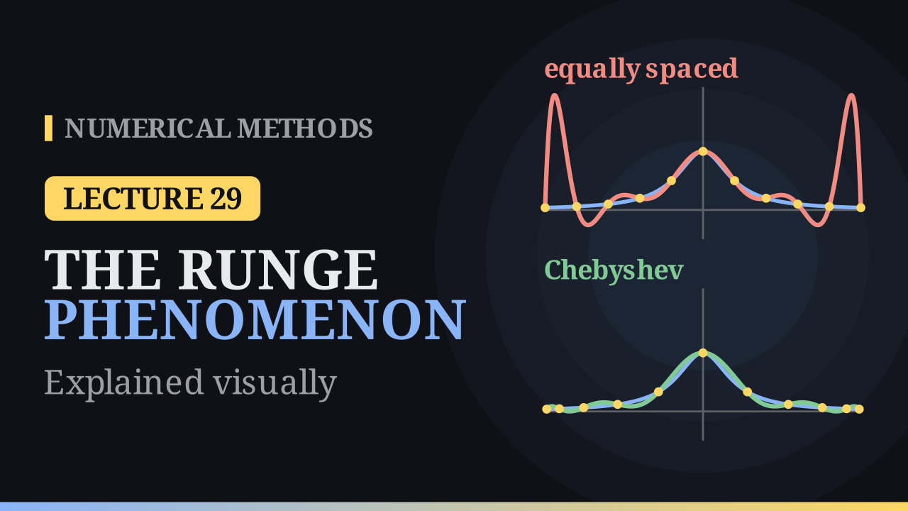
Lecture 29
The Runge Phenomenon
Why more equally spaced nodes can make interpolation worse, and how Chebyshev nodes fix it.
-
07Lectures 30–35 Available
Numerical integration
Trapezoidal and Simpson rules, Gauss–Legendre quadrature
 9:23
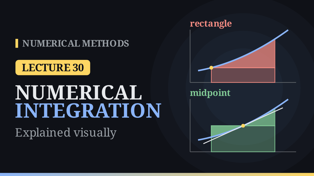
Lecture 30
Introduction to Numerical Integration
Quadrature from interpolation: the rectangle and midpoint rules, their errors, and why the midpoint wins.
 9:18
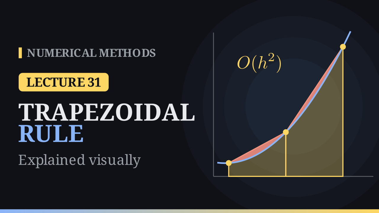
Lecture 31
The Trapezoidal Rule
A straight line through both ends: error h cubed over 12, overestimates of convex functions, and the composite rule of order h squared.
 9:48
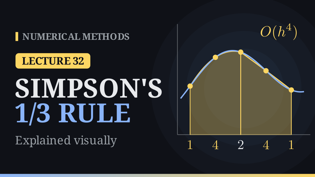
Lecture 32
Simpson's 1/3 Rule
A parabola through three points: weights 1, 4, 1, exact for cubics, and a composite rule whose error falls sixteen times when h is halved.
 9:36
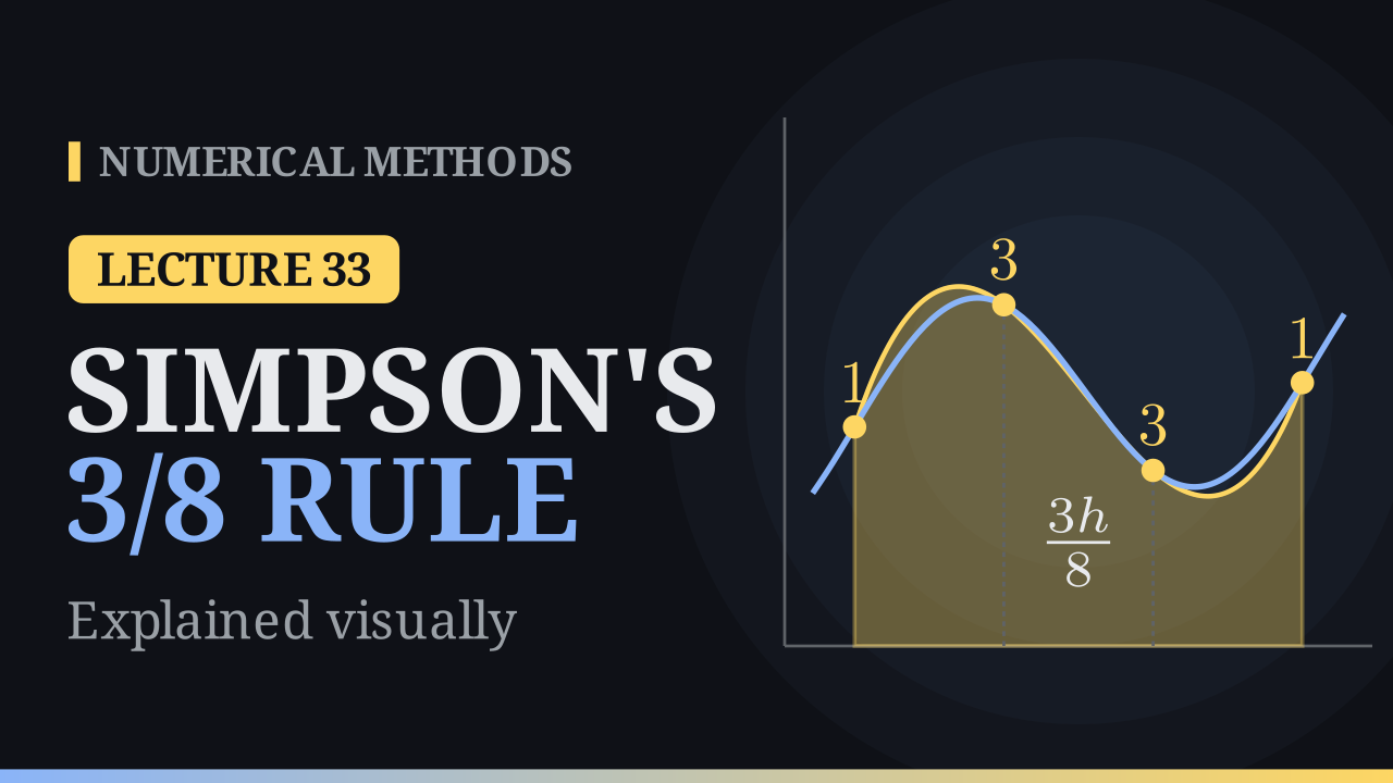
Lecture 33
Simpson's 3/8 Rule
A cubic through four points: weights 1, 3, 3, 1 times 3h/8, the same precision as the 1/3 rule, and the fix for an odd number of pieces.
 13:45
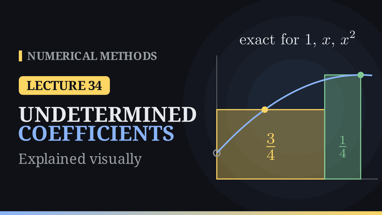
Lecture 34
Method of Undetermined Coefficients
Leave the weights unknown and demand exactness for 1, x, x²: the trapezoid, both Simpson rules and the midpoint rule drop out, plus a rule that never needs f(0).
 14:34
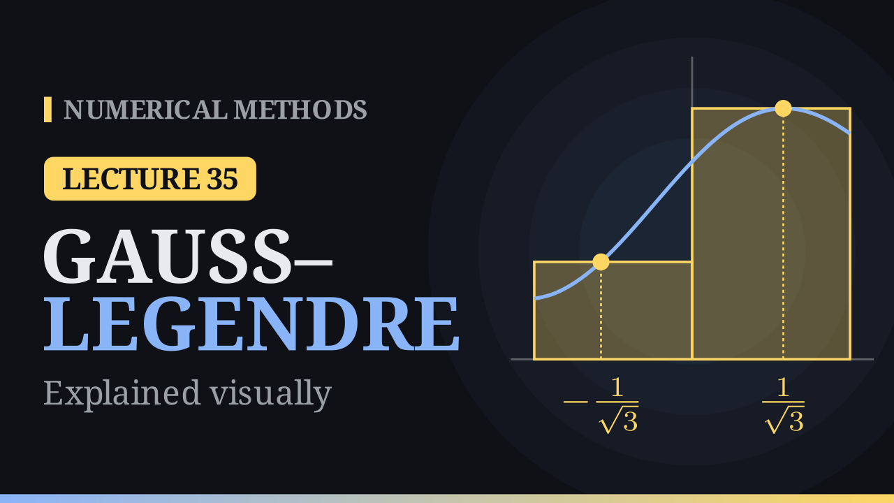
Lecture 35
Gauss–Legendre Quadrature
Free nodes as well as free weights: n points exact for degree 2n − 1, nodes at the roots of the Legendre polynomials, and the most accurate rule per function value.
-
08Lectures 36–42 Available
Differential equations
Euler, Taylor and Runge–Kutta methods, stability and stiffness
 15:31
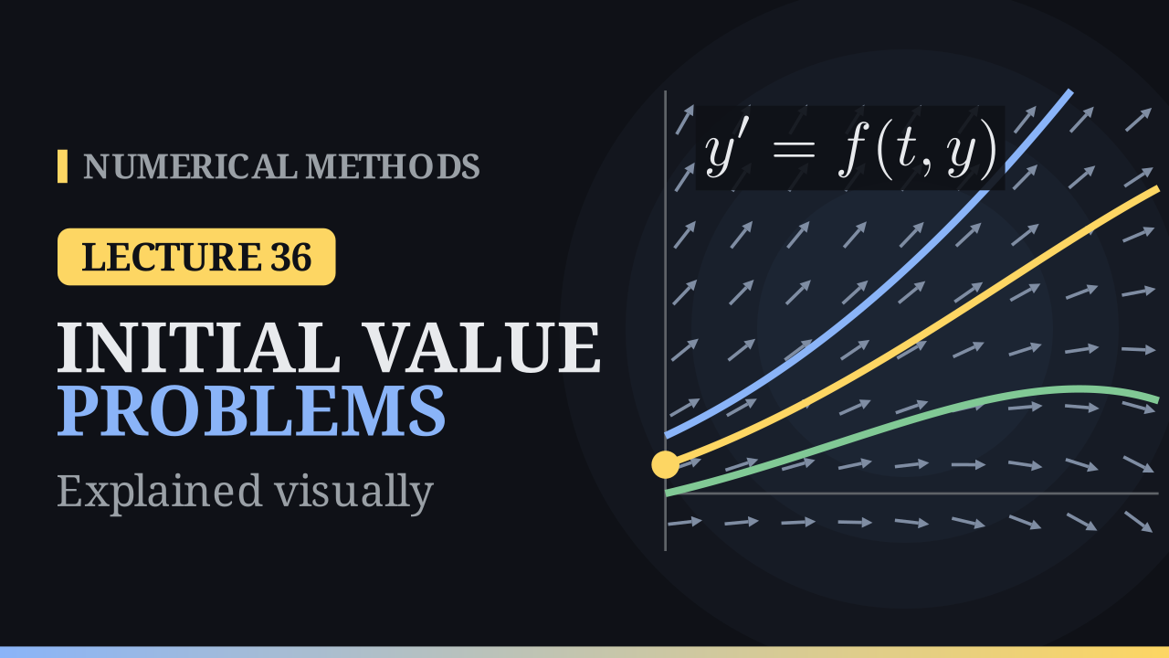
Lecture 36
Initial Value Problems
Direction fields, one curve per initial value, the Lipschitz condition behind existence and uniqueness, and what a numerical method will compute.
 16:45
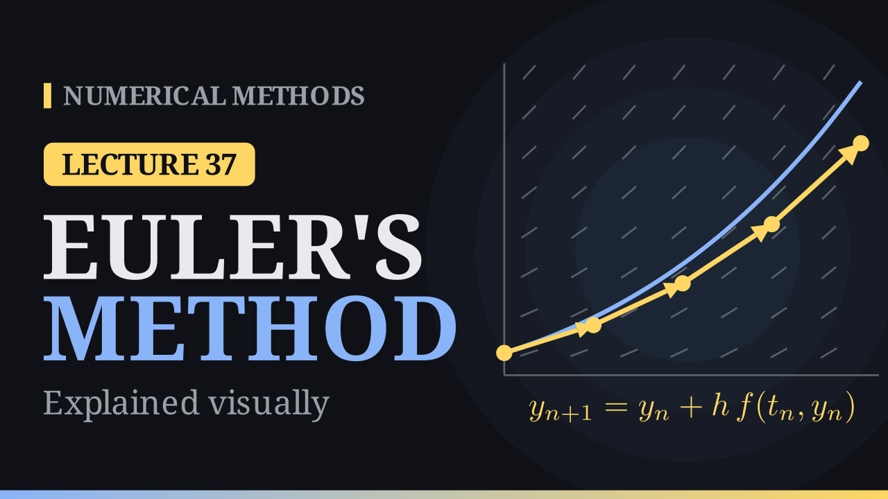
Lecture 37
Euler's Method
Follow the tangent for one step, then repeat: three derivations, local O(h²) against global O(h) error, the stability interval −2 ≤ hλ ≤ 0, and the outward spiral on oscillations.
 16:39
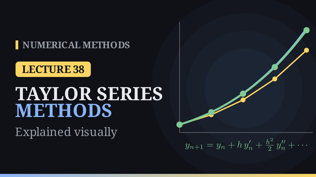
Lecture 38
Taylor Series Methods
Keep more terms of the Taylor series: y″ = f_t + f f_y from the chain rule, order p means global error O(hᵖ), Taylor-2 thirty times more accurate than Euler, and the price of differentiating f.
 17:34
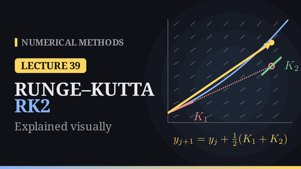
Lecture 39
Runge–Kutta Methods: RK2
Sample the slope twice and blend: Heun and midpoint methods, the order conditions W₁ + W₂ = 1, W₂c₂ = W₂a₂₁ = ½, why two stages stop at order 2, and the error falling by 4 when h is halved.
 18:26
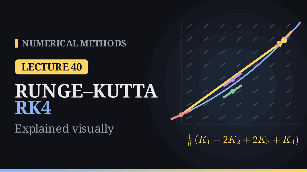
Lecture 40
Runge–Kutta Methods: RK4
Four looks at the slope blended 1, 2, 2, 1 over 6: Simpson's rule for ODEs, global error O(h⁴) so halving h divides the error by 16, fifteen steps where Euler needs millions, and why order 5 needs six stages.
 18:24
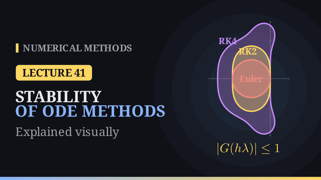
Lecture 41
Stability of Numerical Methods for ODEs
Why an accurate method can still blow up: the growth factor G(hλ), stability regions in the complex plane for Euler, RK2 and RK4, step limits such as h ≤ 2/|λ|, and backward Euler, stable on the whole left half-plane.
 17:37
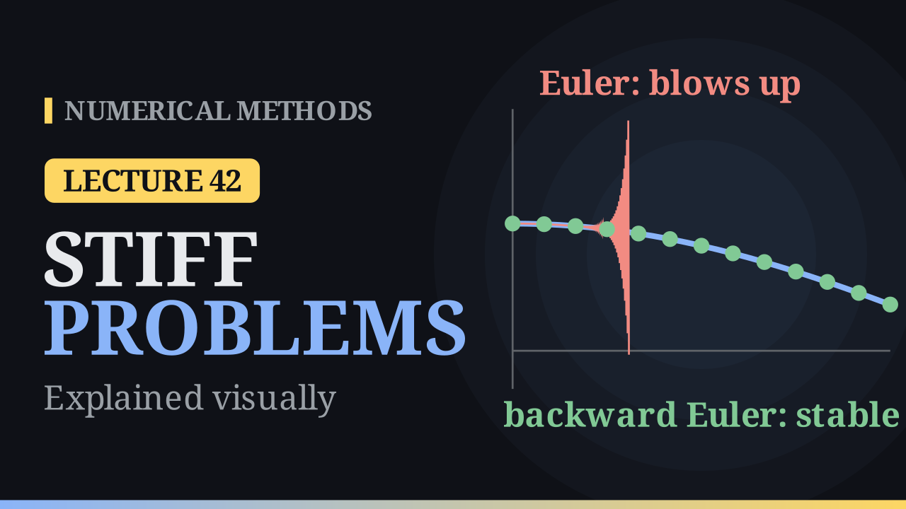
Lecture 42
A-Stability and Stiff Problems
Smooth solutions that explicit methods can't keep up with: A-stability, why explicit Runge–Kutta never is, 100 implicit steps against 5000 Euler steps, and a look back over the whole course.
How each lecture works
Watch, read, practise
- 1
Watch
A 7-minute animated video builds the idea step by step: graphs, worked examples and failure cases.
- 2
Read
The notes collect the formulas, the worked example, the algorithm and the error analysis in one place.
- 3
Practise
Nine short interactive tasks with live plots, hints and instant feedback. Keep a calculator ready (your phone's calculator app is fine). Progress is saved as you go.
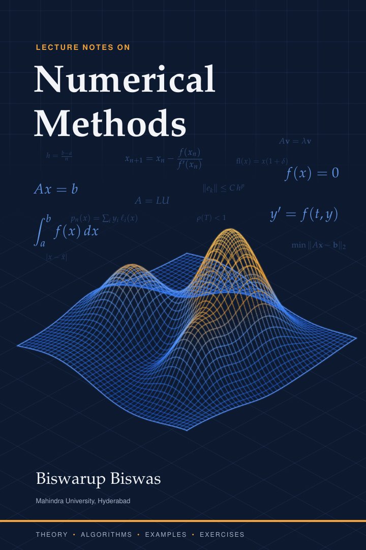
The book
Lecture Notes on Numerical Methods
The notes behind this course are collected in one printed book: theory, algorithms, worked examples and exercises in the same order as the lectures.
Teachers: a specimen copy is available on request.
Start with the bisection method
Lecture 1 introduces the problem of solving \(f(x) = 0\) and the simplest method that always works.
Go to Lecture 1