Lab sheet 3: R Programming
Basic plotting
Create two vectors of same length containing x and y values respectively and then use plot.
x.values <- c(-1.0,-.5,0,0.5,1)
y.values <- c(0,1,2,1.5,1.7)
plot(x.values,y.values)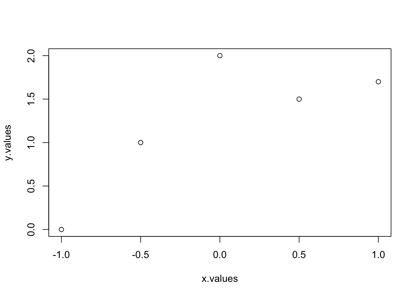
You can also use a matrix whose first column contains x values and second column contains y values.
M<-cbind(x.values,y.values)
plot(M)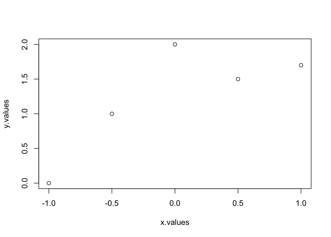
These are some options which can be used in plot.
| type | – | only points or joined by lines or both dots and lines etc. |
| main, xlab, ylab | – | plot title, the horizontal axis label, the vertical axis label |
| col | – | colors of points and line |
| pch | – | character to use for plotting individual points |
| cex | – | the size of plotted point characters |
| lty | – | type of line (for example, solid, dotted, or dashed) |
| lwd | – | the thickness of plotted lines |
| xlim, ylim | – | horizontal and vertical range of the plotting region |
To see the options for these parameter type ?plot in R console and click to Generic X-Y Plotting.
Examples
Let us now see some examples:
plot(x.values,y.values,type="l")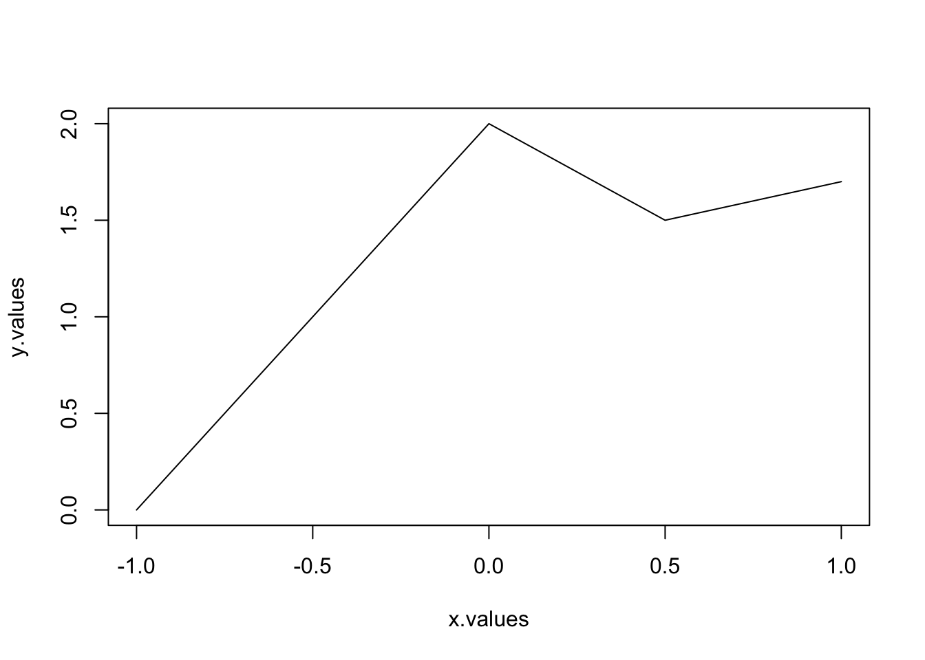
plot(x.values,y.values,type="b")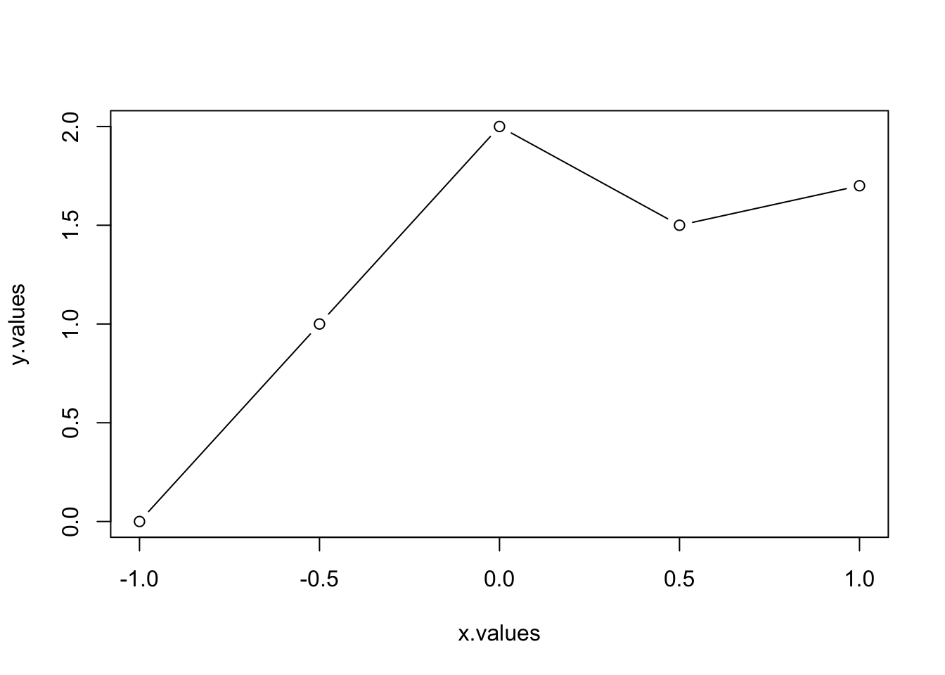
plot(x.values,y.values,type="b",main="My plot title",xlab="x label",
ylab= "y label")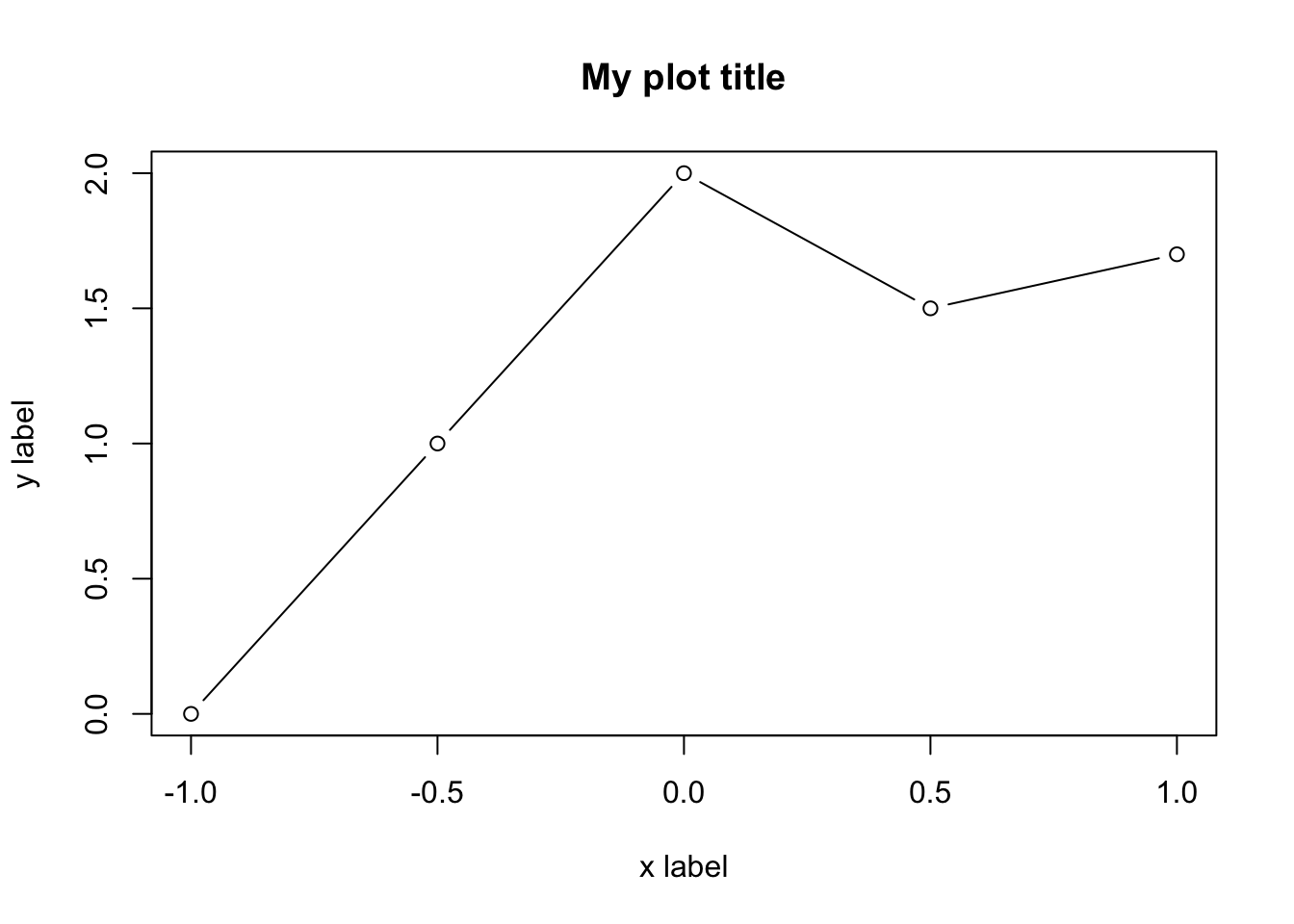
plot(x.values,y.values,type="b",main="My plot title",xlab="x label",
ylab= "y label",col=6,pch=17,lty=1,cex=3,lwd=2,xlim=c(-1,1),ylim=c(0,2))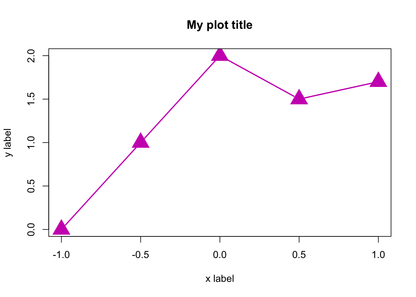
Here are few options for pch:

Adding points, lines, and text in existing plots
We will see the usage of these commands:
| points | – | Adds points |
| lines, abline, segments | – | Adds lines |
| text | – | Writes text |
| arrows | – | Adds arrows |
| legend | – | Adds a legend |
x <- seq(from = -1, to = 20,  length.out = 20)
y <- x*(1-sin(2*pi*x))
plot(x,y,type="p")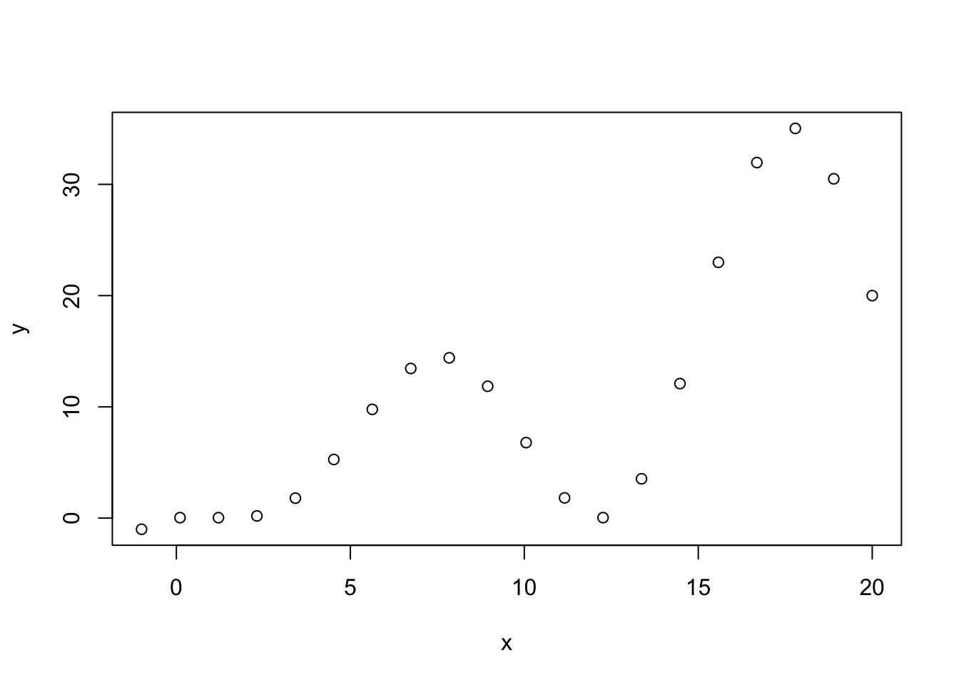
plot(x,y,type="p")
abline(h=c(5,15),col="red",lty=2,lwd=2)
abline(a = 0, b = 1, col = "gray60")
segments(x0=c(5,15),y0=c(15,15),x1=c(5,15),y1=c(5,5),
col=4,lty=4,lwd=2)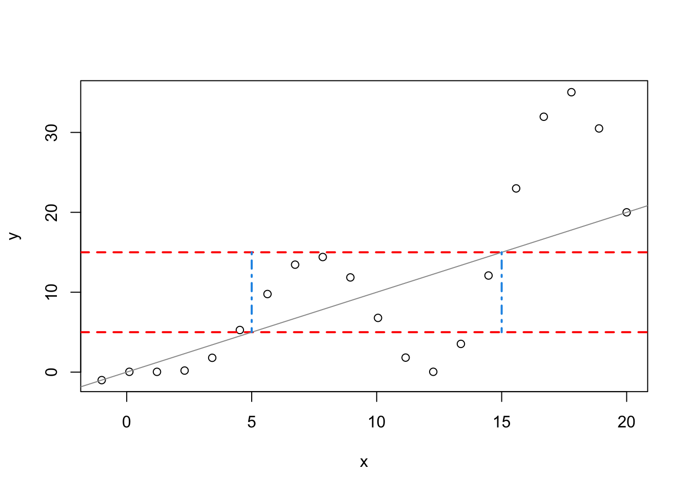
plot(x,y,type="p")
abline(h=c(5,15),col="red",lty=2,lwd=2)
abline(a = 0, b = 1, col = "gray60")
segments(x0=c(5,15),y0=c(15,15),x1=c(5,15),y1=c(5,5),
col=4,lty=4,lwd=2)
points(x[x<=y],y[x<=y],pch=5,col="darkmagenta",cex=2)
points(x[y==max(y)],y[y==max(y)],pch=16,col=10,cex=2)
points(x[(x<=15 & x>=5) & (y<=15 & y>=5)],
y[(x<=15 & x>=5) & (y<=15 & y>=5)],pch=16,col=3,cex=2)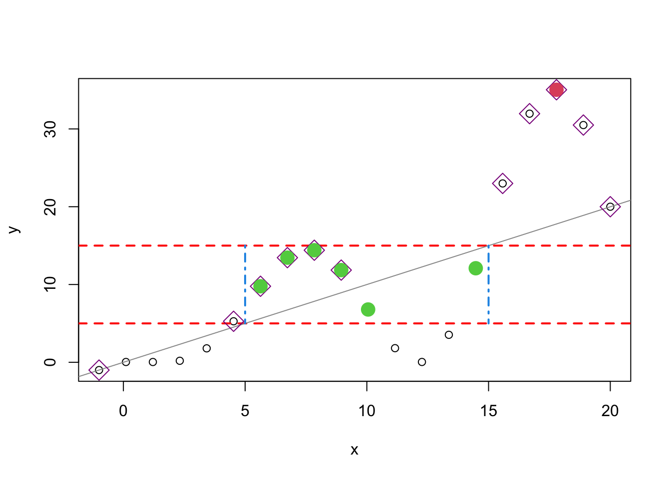
plot(x,y,type="p")
abline(h=c(5,15),col="red",lty=2,lwd=2)
abline(a = 0, b = 1, col = "gray60")
segments(x0=c(5,15),y0=c(15,15),x1=c(5,15),y1=c(5,5),
col=4,lty=4,lwd=2)
points(x[x<=y],y[x<=y],pch=5,col="darkmagenta",cex=2)
points(x[y==max(y)],y[y==max(y)],pch=16,col=10,cex=2)
points(x[(x<=15 & x>=5) & (y<=15 & y>=5)],
y[(x<=15 & x>=5) & (y<=15 & y>=5)],pch=16,col=3,cex=2)
lines(x,y,lty=4)
arrows(x0=8,y0=25,x1=17,y1=35)
text(x=8,y=25,pos=1,labels="the highest peak")
legend("topleft",
legend=c("main curve","two horizontal line","x=y line",
"above x=y line","favourable points"),pch=c(1,NA,NA,5,16),lty=c(4,2,1,NA,NA),
col=c("black","red","gray60","darkmagenta",3),
lwd=c(1,2,1,1,NA),pt.cex=c(1,NA,NA,2,2))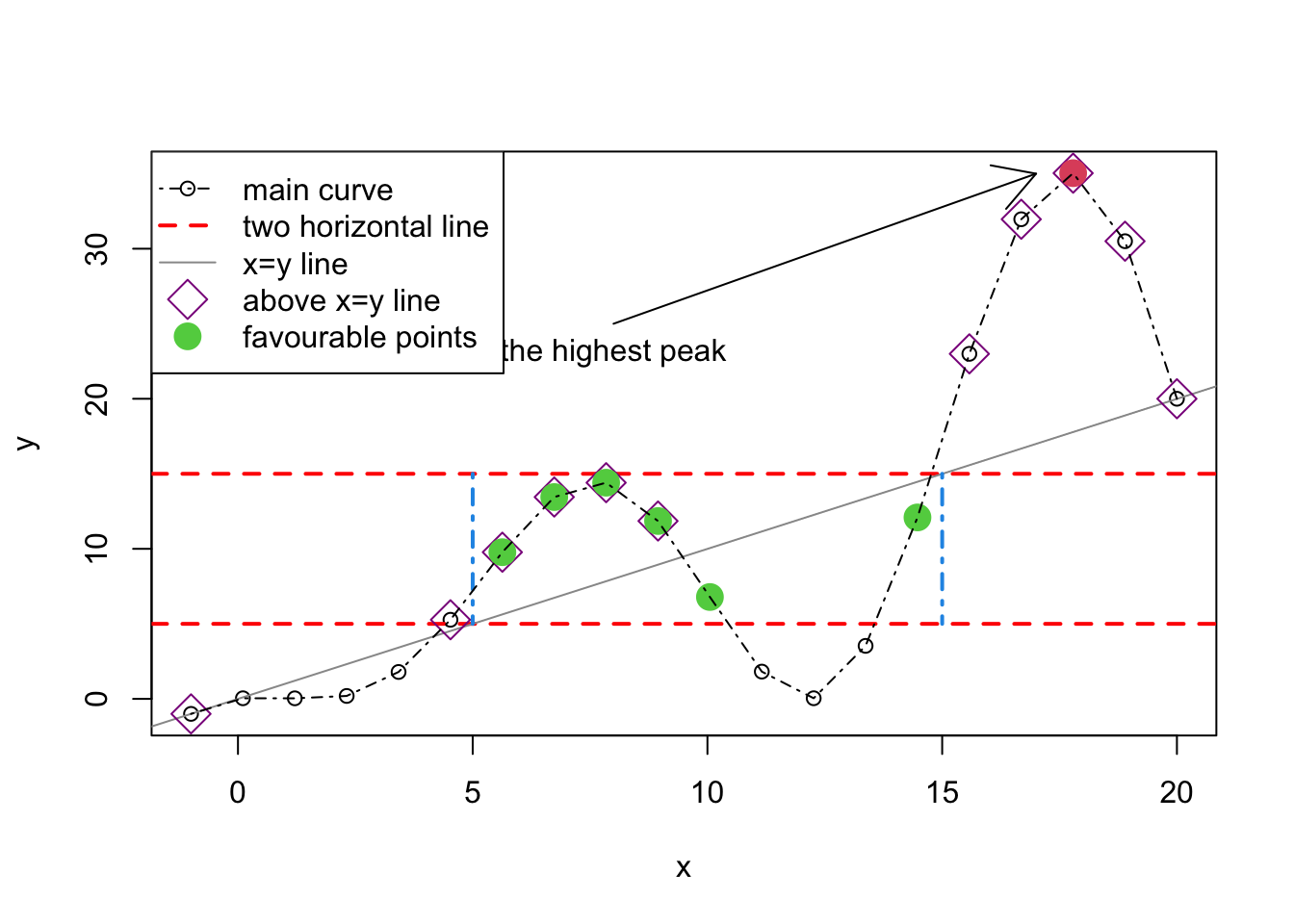
Shading between curves
x1=seq(from=-pi,to=pi,length.out =100)
y1 <- sin(x1)
y2 <- cos(x1)
plot(x1,y1,type="l",bty="L",xlab="x",ylab="y",col=4)
points(x1,y2,type="l",col="red")
polygon(c(x1,rev(x1)),c(y2,rev(y1)),col=gray(0.8))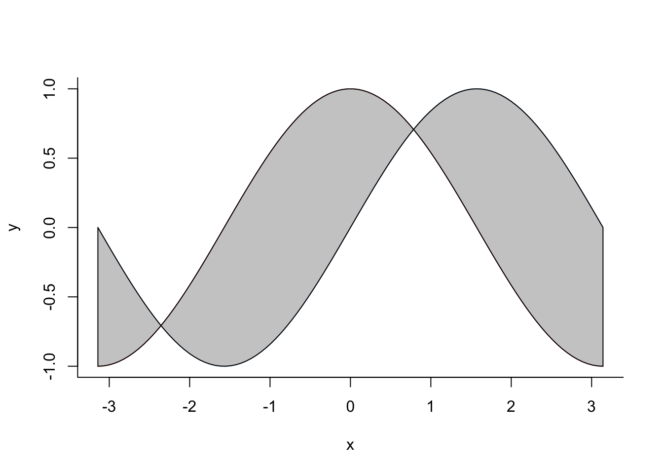
plot(x,y,type="n")
rect(5, 5, 15, 15, col=gray(0.9), border=NA)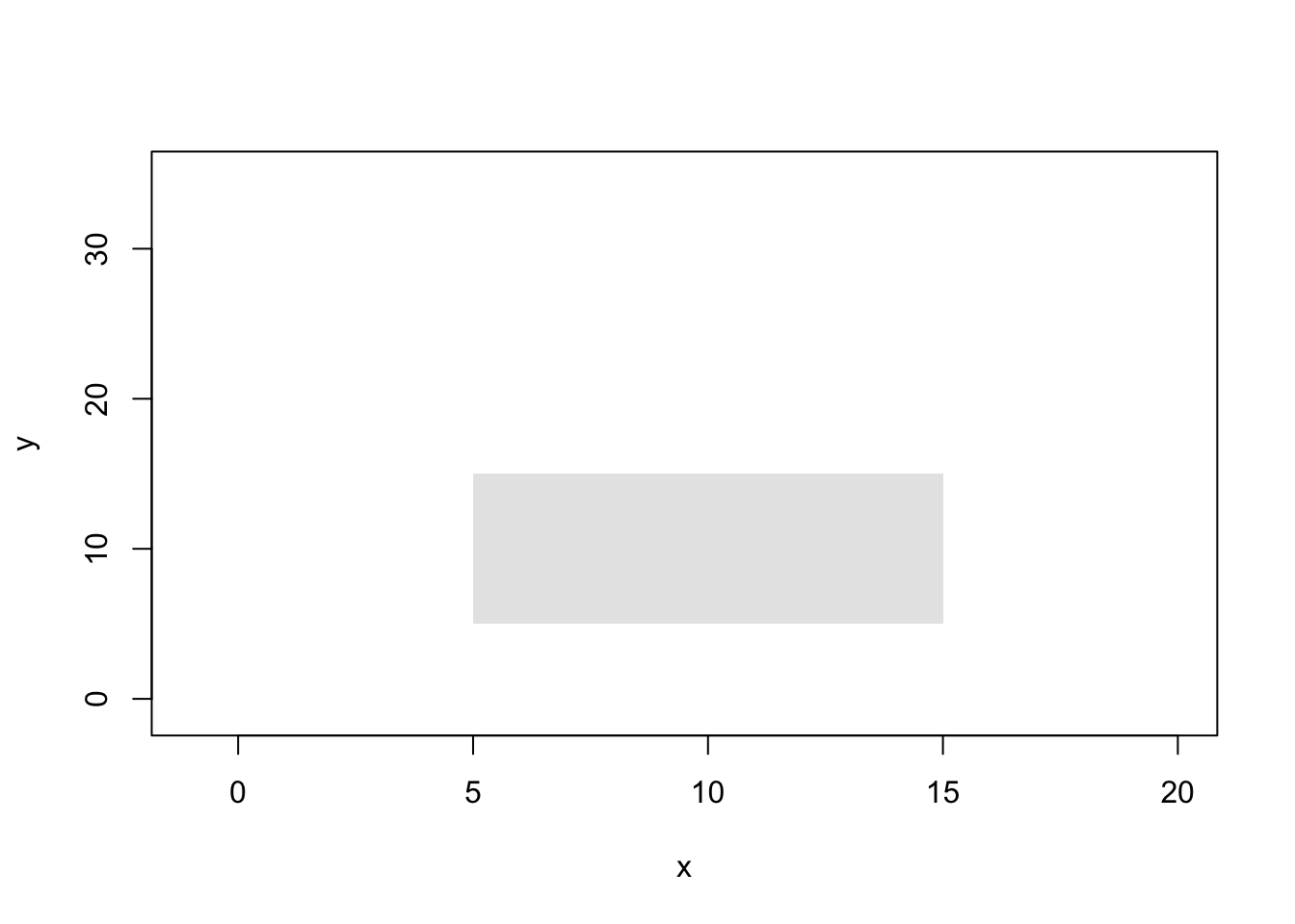
Packages other than R base
There are few good R packages for data visualisation: ggplot2, Lattice, Plotly and few more. Let us explore ggplot2 a bit. First, use install.packages(``ggplot2”) to install.
library("ggplot2")
qplot(x.values,y.values)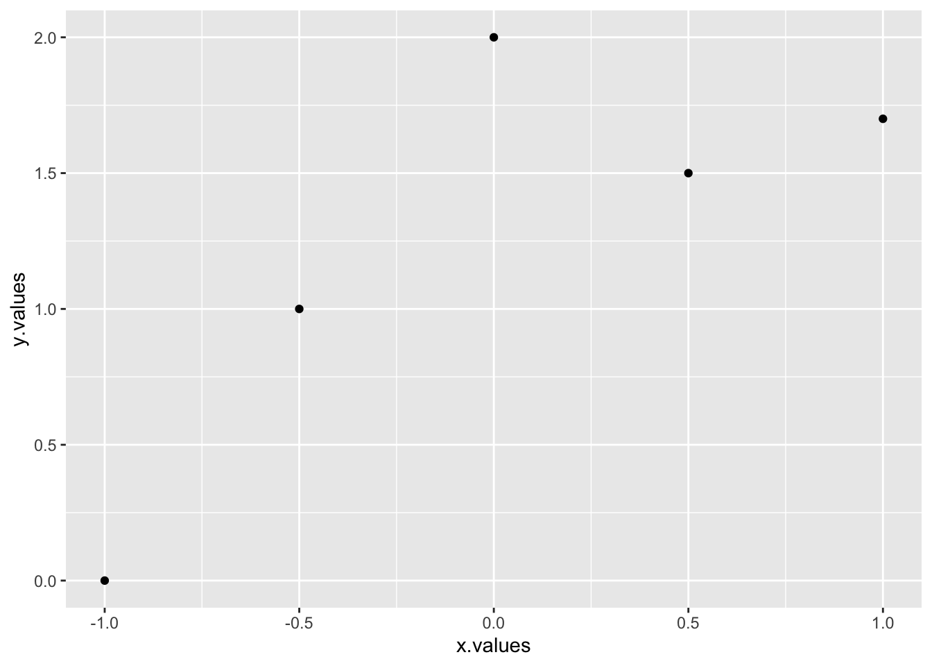
qplot(x.values,y.values,main="My qplot",xlab="x label",
ylab= "y label")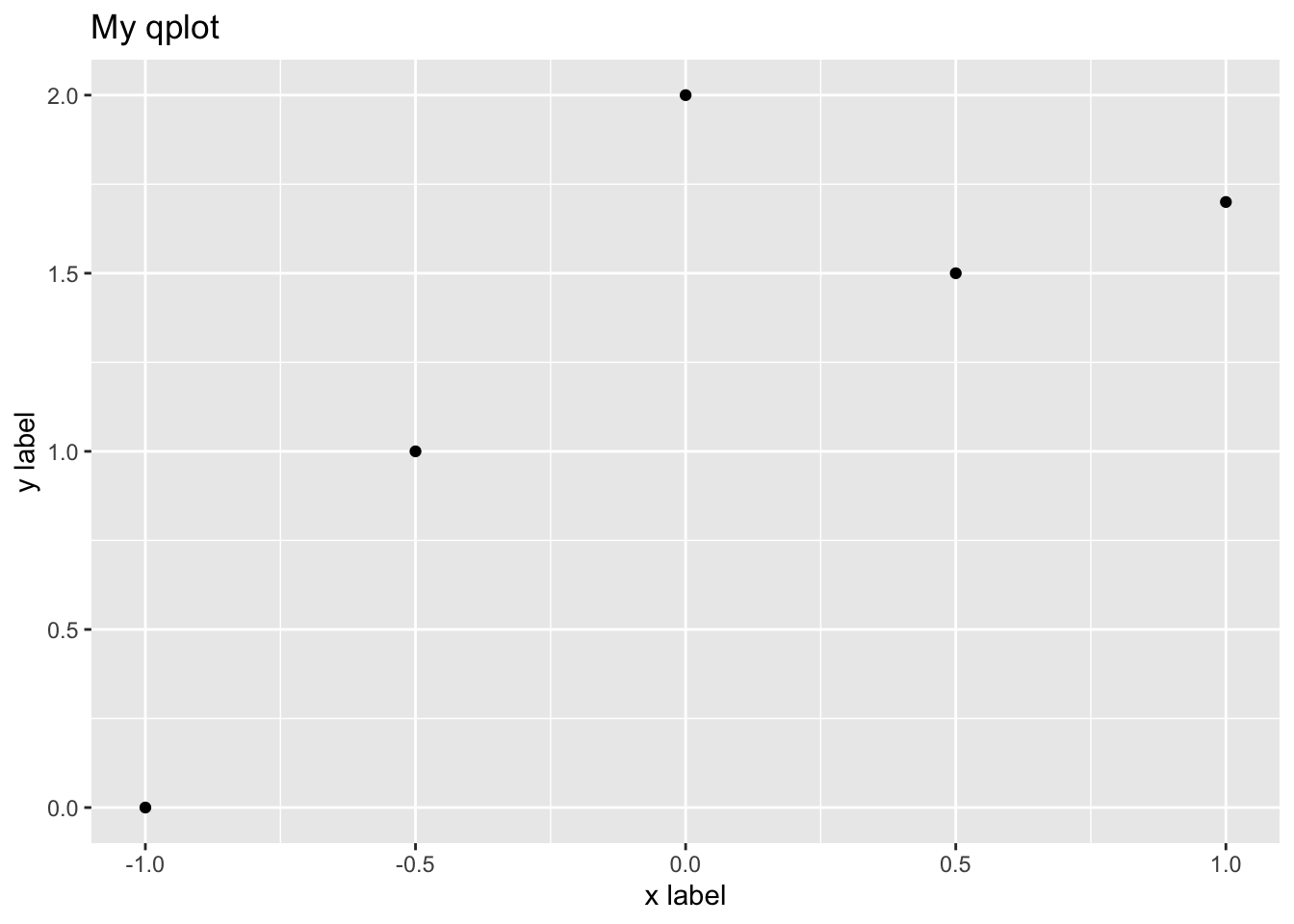
h=qplot(x.values,y.values)
h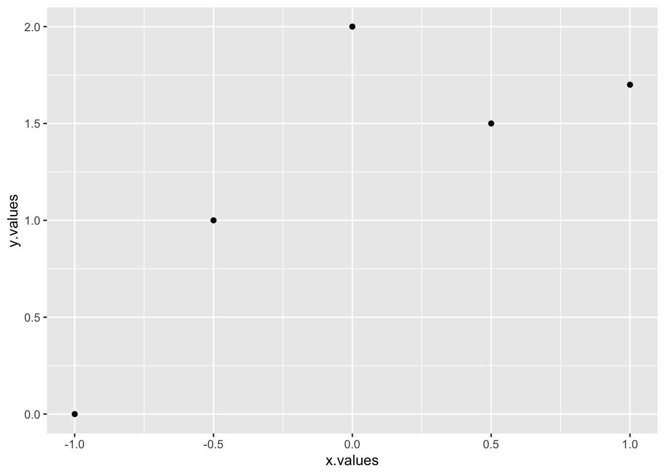
qplot(x,y,geom="blank") + geom_point() + geom_line()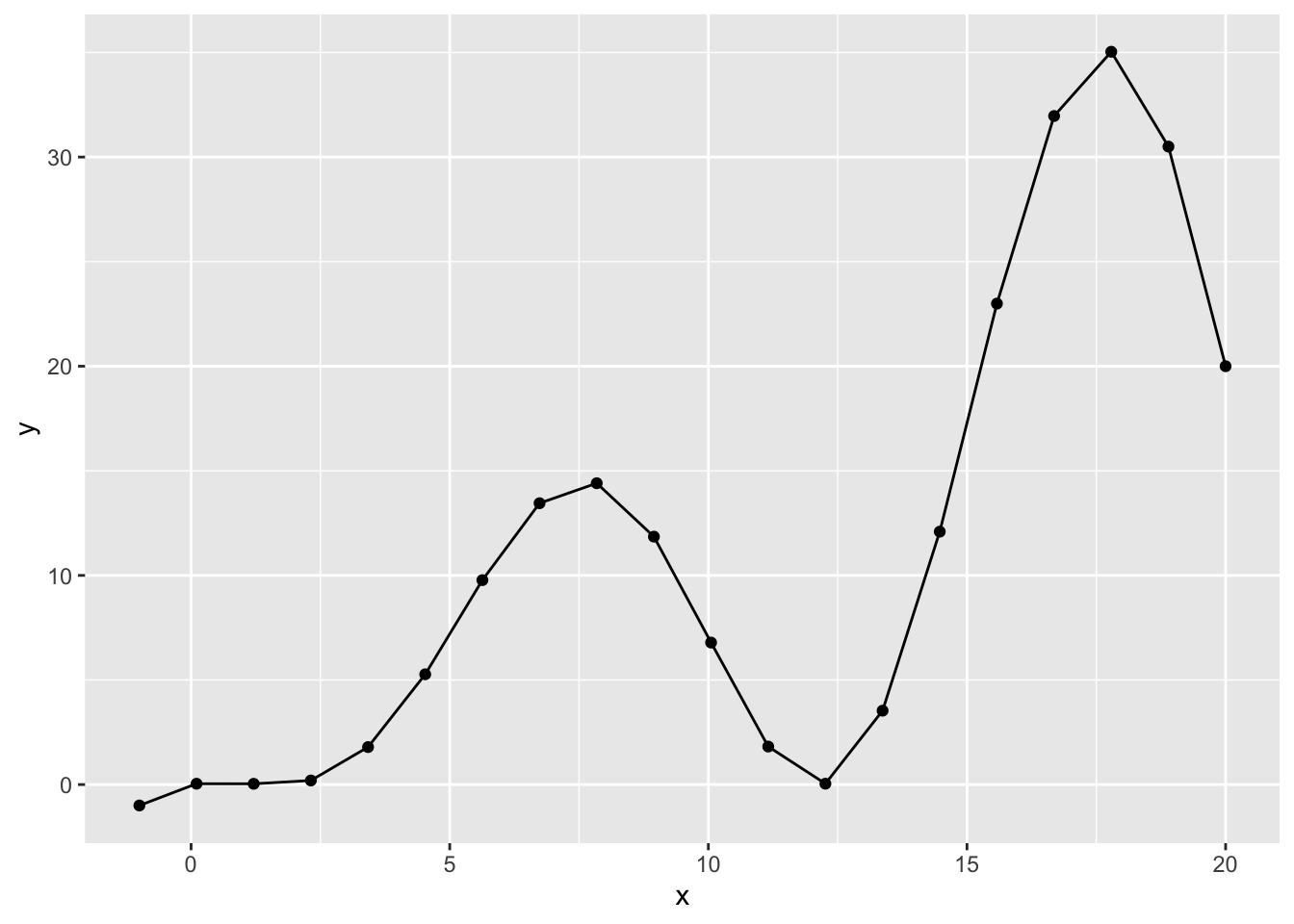
myqplot <- qplot(x,y,geom="blank") + geom_line(color="red",linetype=2) +
geom_point(size=3,shape=3,color="blue")
myqplot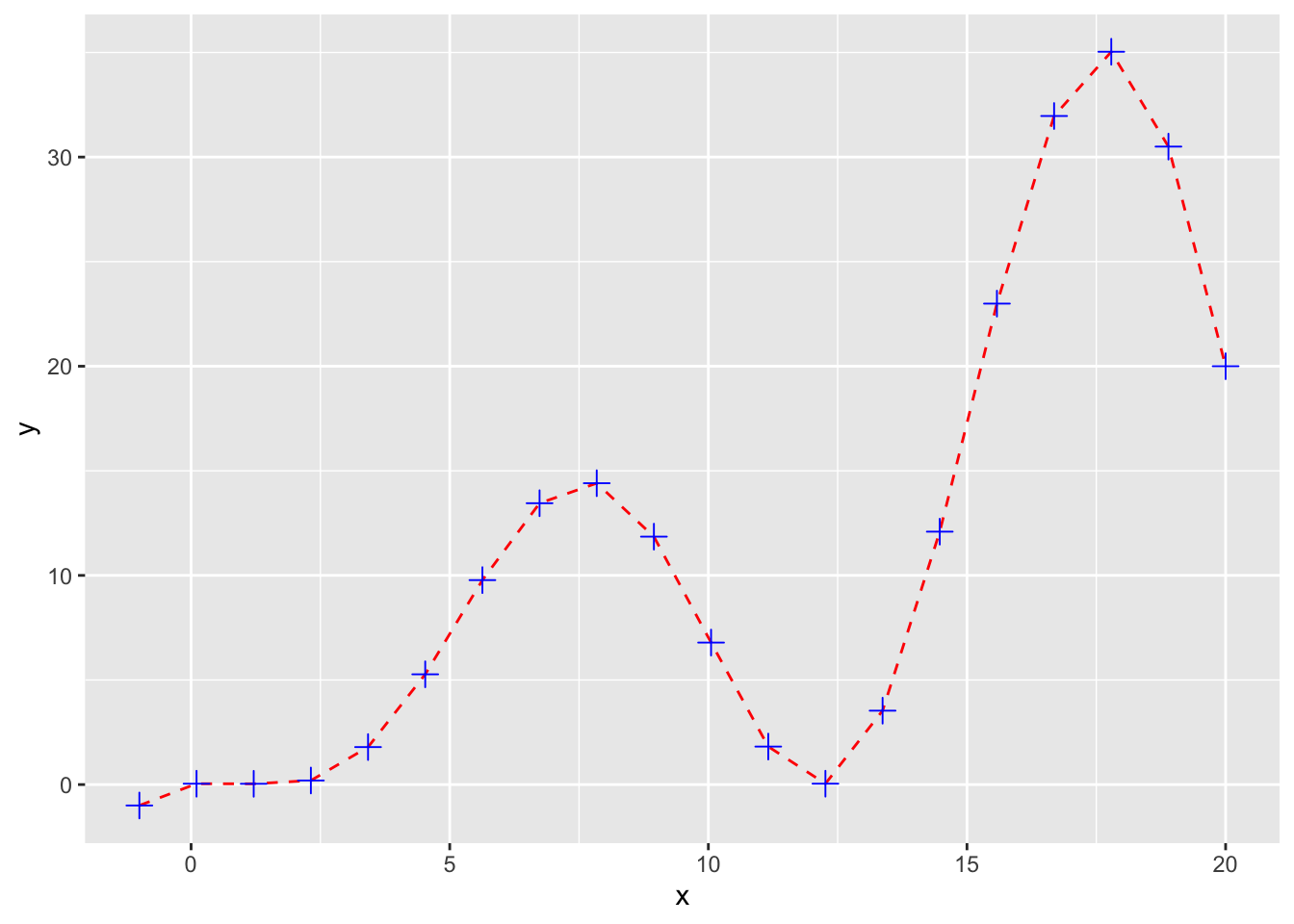
ptype <- rep("other",length(x=x))
ptype[x<=y] <- "x<=y"
ptype[(x<=15 & x>=5) & (y<=15 & y>=5)] <- "favourable"
ptype[y==max(y)]<-"peak"
ptype <- factor(x=ptype)
ptype
## [1] x<=y other other other other x<=y
## [7] favourable favourable favourable favourable favourable other
## [13] other other favourable x<=y x<=y peak
## [19] x<=y x<=y
## Levels: favourable other peak x<=yqplot(x,y,color=ptype,shape=ptype)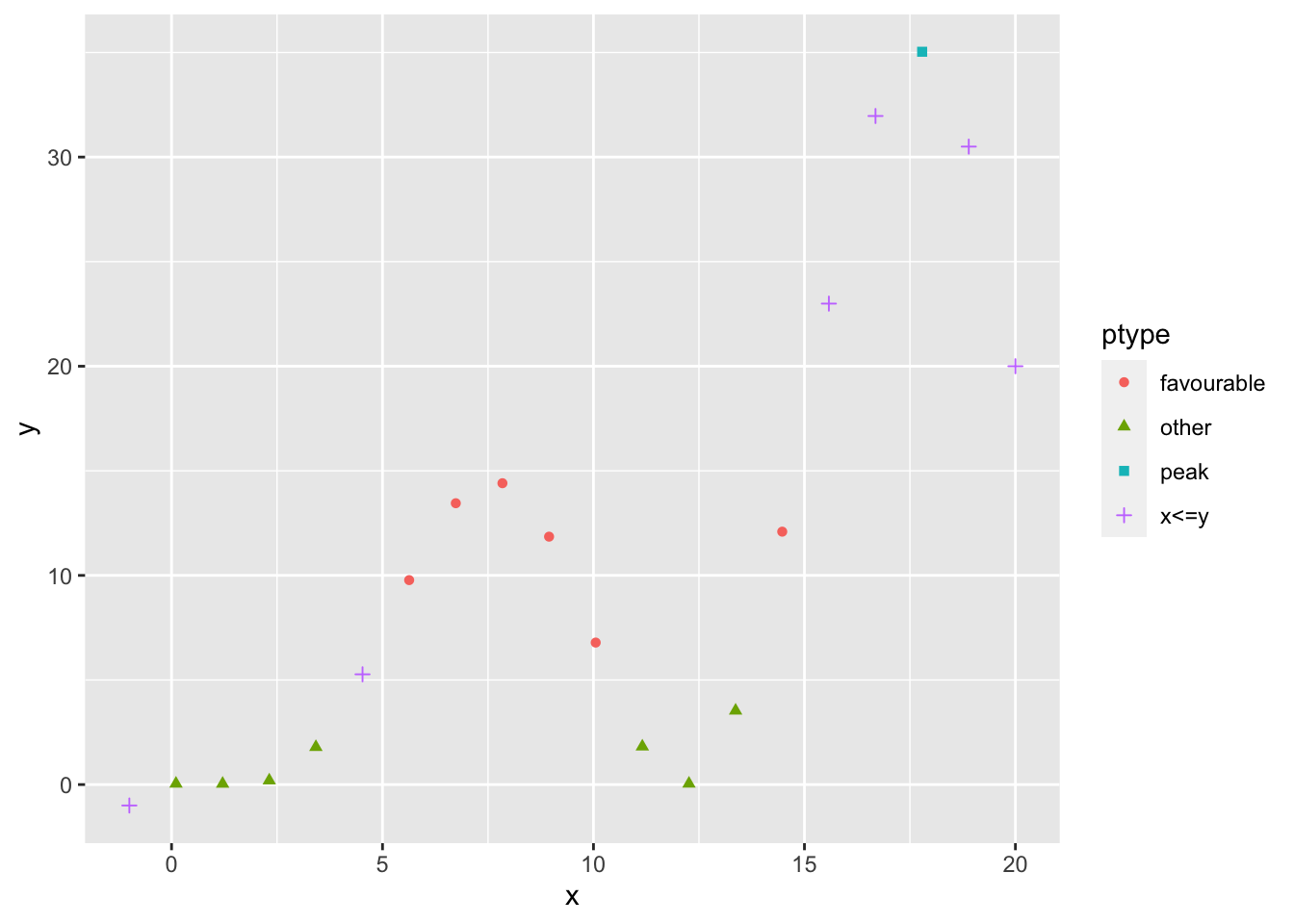
qplot(x,y,color=ptype,shape=ptype) + geom_point(size=4) +
geom_line(mapping=aes(group=1),color="black",lty=2) +
geom_hline(mapping=aes(yintercept=c(5,15)),color="red")+
geom_segment(mapping=aes(x=5,y=5,xend=5,yend=15),color="red",lty=3)+
geom_segment(mapping=aes(x=15,y=5,xend=15,yend=15),color="red",lty=3)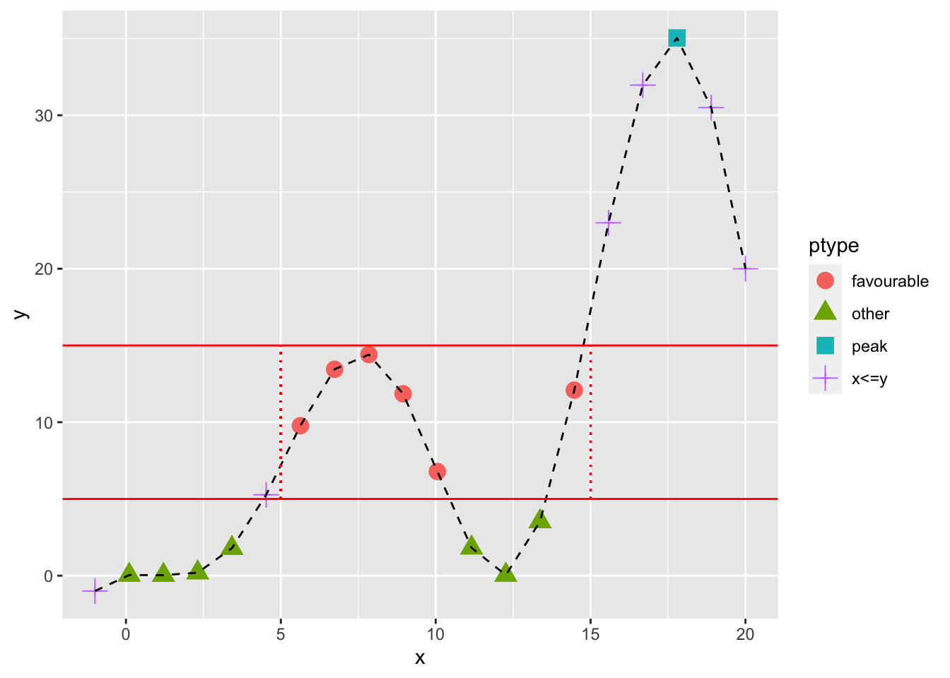
x1=seq(from=-pi,to=pi,length.out =100)
y1 <- sin(x1)
y2 <- cos(x1)
mydata=data.frame(x=x1,sin=y1,cos=y2)
ggplot(data = mydata)+
geom_ribbon(aes(x=x, ymax=cos, ymin=sin), fill="gray")+
geom_line(aes(x=x,y = sin), colour = 'red') +
geom_line(aes(x=x,y = cos), colour = 'blue')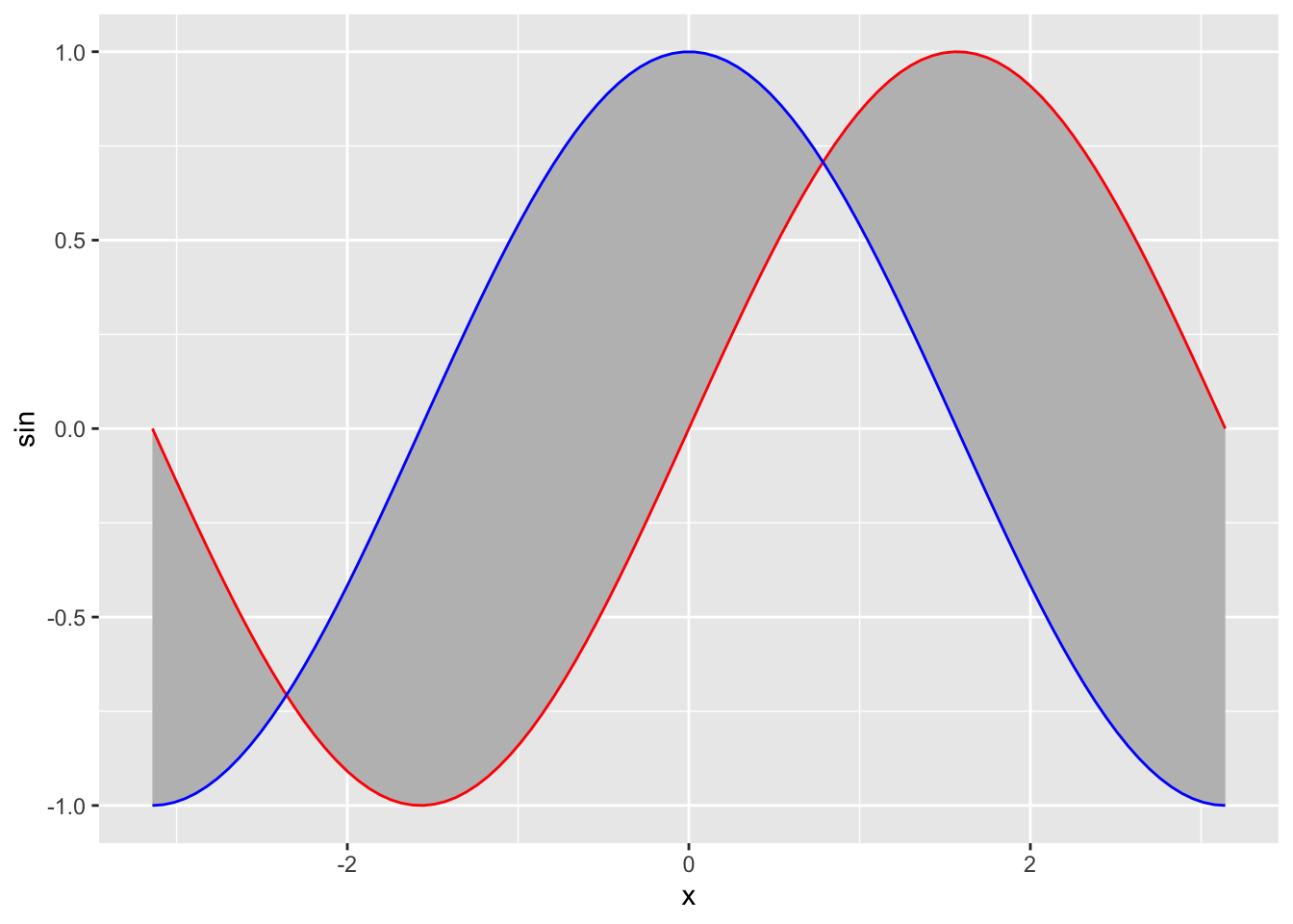
Package plotly
Basic Scatter Plot
library(ggplot2)
library(plotly)
##
## Attaching package: 'plotly'## The following object is masked from 'package:ggplot2':
##
## last_plot## The following object is masked from 'package:stats':
##
## filter## The following object is masked from 'package:graphics':
##
## layoutfig <- plot_ly(data = iris, x = ~Sepal.Length, y = ~Petal.Length)
fig## No trace type specified:
## Based on info supplied, a 'scatter' trace seems appropriate.
## Read more about this trace type -> https://plotly.com/r/reference/#scatter## No scatter mode specifed:
## Setting the mode to markers
## Read more about this attribute -> https://plotly.com/r/reference/#scatter-modePlotting Markers and Lines
library(plotly)
trace_0 <- rnorm(100, mean = 5)
trace_1 <- rnorm(100, mean = 0)
trace_2 <- rnorm(100, mean = -5)
x <- c(1:100)
data <- data.frame(x, trace_0, trace_1, trace_2)
fig <- plot_ly(data, x = ~x)
fig <- fig %>% add_trace(y = ~trace_0, name = 'trace 0',mode = 'lines')
fig <- fig %>% add_trace(y = ~trace_1, name = 'trace 1', mode = 'lines+markers')
fig <- fig %>% add_trace(y = ~trace_2, name = 'trace 2', mode = 'markers')
fig## No trace type specified:
## Based on info supplied, a 'scatter' trace seems appropriate.
## Read more about this trace type -> https://plotly.com/r/reference/#scatter
## No trace type specified:
##   Based on info supplied, a 'scatter' trace seems appropriate.
##   Read more about this trace type -> https://plotly.com/r/reference/#scatter
## No trace type specified:
## Based on info supplied, a 'scatter' trace seems appropriate.
## Read more about this trace type -> https://plotly.com/r/reference/#scatterQualitative Colorscales
library(plotly)

fig <- plot_ly(data = iris, x = ~Sepal.Length, y = ~Petal.Length, color = ~Species)

fig
## No trace type specified:
## Based on info supplied, a 'scatter' trace seems appropriate.
## Read more about this trace type -> https://plotly.com/r/reference/#scatter## No scatter mode specifed:
## Setting the mode to markers
## Read more about this attribute -> https://plotly.com/r/reference/#scatter-modeAdding Color and Size Mapping
library(plotly)

d <- diamonds[sample(nrow(diamonds), 1000), ]

fig <- plot_ly(
  d, x = ~carat, y = ~price,
  color = ~carat, size = ~carat
)
fig
## No trace type specified:
## Based on info supplied, a 'scatter' trace seems appropriate.
## Read more about this trace type -> https://plotly.com/r/reference/#scatter## No scatter mode specifed:
## Setting the mode to markers
## Read more about this attribute -> https://plotly.com/r/reference/#scatter-modeFilling between curves
library(ggplot2)
library(plotly)
x1=seq(from=-pi,to=pi,length.out =100)
y1 <- sin(x1)
y2 <- cos(x1)
mydata=data.frame(x=x1,sin=y1,cos=y2)
fig1 <- mydata %>%
  plot_ly(
    x = ~x1,
    y = ~y1,
    type = 'scatter',
    mode = 'lines',
    showlegend = F
  )
fig1 <- fig1 %>% add_trace(x=x1,y=y2,fill = 'tonexty')
fig1
Animation
library(ggplot2)
library(plotly)

x.seq <- seq(from=-10,to=10,length.out=100)

sigma <- 1
mu <- 0
y.seq <- (1/sqrt(2*pi)/sigma)*exp(-(x.seq-mu)^2/(2*sigma^2))
data=data.frame(xseq=x.seq,yseq=y.seq,sigma=sigma)

for (i in 1:20){
  sigma <- sigma+0.1
  y.seq <- (1/sqrt(2*pi)/sigma)*exp(-(x.seq-mu)^2/(2*sigma^2))
  newdata=data.frame(xseq=x.seq,yseq=y.seq,sigma=sigma)
  data=rbind(data,newdata)
}

fig <- data %>%
  plot_ly(
    x = ~xseq,
    y = ~yseq,
    frame = ~sigma,
    type = 'scatter',
    mode = 'lines',
    showlegend = F
  )
fig
References
Look into the following for more on line and scatter plot. https://plotly.com/r/line-and-scatter/